Variance partitioning analysis

Developed by Gabriel Hoffman

Run on 2024-02-07 12:08:50

Introduction

Gene expression datasets are complicated and have multiple sources of biological and technical variation. These datasets have recently become more complex as it is now feasible to assay gene expression from the same individual in multiple tissues or at multiple time points. The variancePartition package implements a statistical method to quantify the contribution of multiple sources of variation and decouple within/between-individual variation. In addition, variancePartition produces results at the gene-level to identity genes that follow or deviate from the genome-wide trend.

The variancePartition package provides a general framework for understanding drivers of variation in gene expression in experiments with complex designs. A typical application would consider a dataset of gene expression from individuals sampled in multiple tissues or multiple time points where the goal is to understand variation within versus between individuals and tissues. variancePartition use a linear mixed model to partition the variance attributable to multiple variables in the data. The analysis is built on top of the lme4 package (Bates et al. 2015), and some basic knowledge about linear mixed models will give you some intuition about the behavior of variancePartition (Pinheiro and Bates 2000; Galecki and Burzykowski 2013).

Input data

There are three components to an analysis:

1. Gene expression data: In general, this is a matrix of normalized gene expression values with genes as rows and experiments as columns.

• Count-based quantification: featureCounts (Liao, Smyth, and Shi 2014), HTSeq (Anders, Pyl, and Huber 2015)

  Counts mapping to each gene can be normalized using counts per million (CPM), reads per kilobase per million (RPKM) or fragments per kilobase per million (FPKM). These count results can be processed with limma::voom() (Law et al. 2014) to model the precision of each observation or DESeq2 (Love, Huber, and Anders 2014).

• Isoform quantification: kallisto (Bray et al. 2016), sailfish (Patro, Mount, and Kingsford 2014), salmon (Patro, Duggal, and Kingsford 2015), RSEM (Li and Dewey 2011), cufflinks (Trapnell et al. 2010)

  These perform isoform-level quantification using reads that map to multiple transcripts. Quantification values can be read directly into R, or processed with ballgown (Frazee et al. 2015) or tximport (Soneson, Love, and Robinson 2015).

• Microarray data: any standard normalization such as rma in the oligo (Carvalho and Irizarry 2010) package can be used.

• Any set of features: chromatin accessibility, protein quantification, etc

2. Metadata about each experiment:

   A data.frame with information about each experiment such as patient ID, tissue, sex, disease state, time point, batch, etc.

3. Formula indicating which metadata variables to consider:

   An R formula such as ~ Age + (1|Individual) + (1|Tissue) + (1|Batch) indicating which metadata variables should be used in the analysis.

Variance partitioning analysis will assess the contribution of each metadata variable to variation in gene expression and can report the intra-class correlation for each variable.

Running an analysis

A typical analysis with variancePartition is only a few lines of R code, assuming the expression data has already been normalized. Normalization is a separate topic addressed briefly in [Applying variancePartition to RNA-seq expression data].

The simulated dataset included as an example contains measurements of 200 genes from 100 samples. These samples include assays from 3 tissues across 25 individuals processed in 4 batches. The individuals range in age from 36 to 73. A typical variancePartition analysis will assess the contribution of each aspect of the study design (i.e. individual, tissue, batch, age) to the expression variation of each gene. The analysis will prioritize these axes of variation based on a genome-wide summary and give results at the gene-level to identity genes that follow or deviate from this genome-wide trend. The results can be visualized using custom plots and can be used for downstream analysis.

Standard application

# load library
library("variancePartition")

# load simulated data:
# geneExpr: matrix of gene expression values
# info: information/metadata about each sample
data(varPartData)

# Specify variables to consider
# Age is continuous so model it as a fixed effect
# Individual and Tissue are both categorical,
# so model them as random effects
# Note the syntax used to specify random effects
form <- ~ Age + (1 | Individual) + (1 | Tissue) + (1 | Batch)

# Fit model and extract results
# 1) fit linear mixed model on gene expression
# If categorical variables are specified,
#     a linear mixed model is used
# If all variables are modeled as fixed effects,
#       a linear model is used
# each entry in results is a regression model fit on a single gene
# 2) extract variance fractions from each model fit
# for each gene, returns fraction of variation attributable
#       to each variable
# Interpretation: the variance explained by each variables
# after correcting for all other variables
# Note that geneExpr can either be a matrix,
# and EList output by voom() in the limma package,
# or an ExpressionSet
varPart <- fitExtractVarPartModel(geneExpr, form, info)

# sort variables (i.e. columns) by median fraction
#       of variance explained
vp <- sortCols(varPart)

# Figure 1a
# Bar plot of variance fractions for the first 10 genes
plotPercentBars(vp[1:10, ])

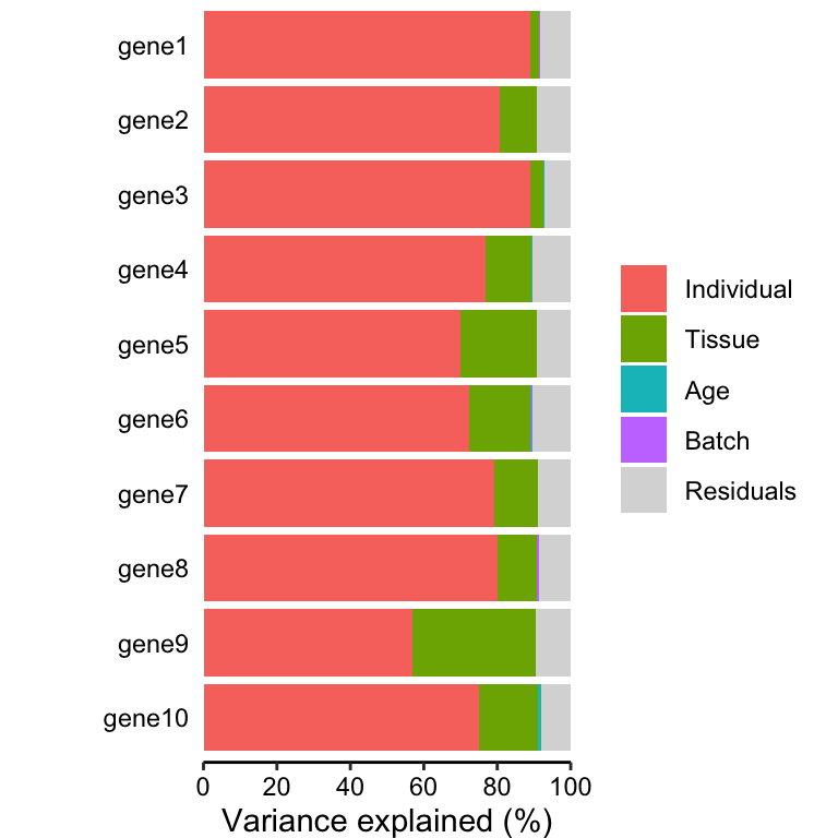
# Figure 1b
# violin plot of contribution of each variable to total variance
plotVarPart(vp)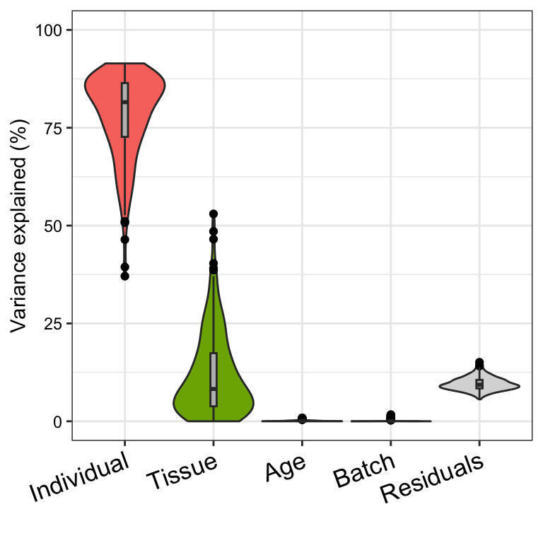

variancePartition includes a number of custom plots to visualize the results. Since variancePartition attributes the fraction of total variation attributable to each aspect of the study design, these fractions naturally sum to 1. plots the partitioning results for a subset of genes (Figure 1a), and shows a genome-wide violin plot of the distribution of variance explained by each variable across all genes (Figure 1b). (Note that these plots show results in terms of of variance explained, while the results are stored in terms of the fraction.)

The core functions of variancePartition work seemlessly with gene expression data stored as a matrix, data.frame, EList from limma or ExpressionSet from Biobase. fitExtractVarPartModel() returns an object that stores the variance fractions for each gene and each variable in the formula specified. These fractions can be accessed just like a data.frame:

# Access first entries
head(varPart)

##             Batch Individual     Tissue          Age  Residuals
## gene1 0.000157945  0.8903733 0.02468893 4.528906e-05 0.08473455
## gene2 0.000000000  0.8060314 0.10101922 3.336680e-04 0.09261567
## gene3 0.002422174  0.8901096 0.03562102 1.471701e-03 0.07037550
## gene4 0.000000000  0.7688278 0.12531362 1.014413e-03 0.10484419
## gene5 0.000000000  0.6997242 0.20910139 3.871485e-05 0.09113569
## gene6 0.002343666  0.7222283 0.16786542 2.717378e-03 0.10484521

# Access first entries for Individual
head(varPart$Individual)

## [1] 0.8903733 0.8060314 0.8901096 0.7688278 0.6997242 0.7222283

# sort genes based on variance explained by Individual
head(varPart[order(varPart$Individual, decreasing = TRUE), ])

##               Batch Individual      Tissue          Age  Residuals
## gene43  0.000000000  0.9143523 0.011737153 3.776742e-04 0.07353289
## gene174 0.000000000  0.9112702 0.009726001 2.015102e-03 0.07698865
## gene111 0.000000000  0.9067082 0.008386574 9.735963e-04 0.08393165
## gene127 0.000000000  0.9035627 0.013838828 5.081822e-04 0.08209028
## gene151 0.006079206  0.9029393 0.000000000 1.345019e-05 0.09096803
## gene91  0.000000000  0.9002946 0.014144910 1.110514e-06 0.08555939

Saving plot to file

In order to save the plot to a file, use the ggsave() function:

fig <- plotVarPart(vp)
ggsave(file, fig)

Plot expression stratified by other variables

variancePartition also includes plotting functions to visualize the variation across a variable of interest. plots the expression of a gene stratified by the specified variable. In the example dataset, users can plot a gene expression trait stratified by Tissue (Figure 2a) or Individual (Figure 2b).

# get gene with the highest variation across Tissues
# create data.frame with expression of gene i and Tissue
#       type for each sample
i <- which.max(varPart$Tissue)
GE <- data.frame(Expression = geneExpr[i, ], Tissue = info$Tissue)

# Figure 2a
# plot expression stratified by Tissue
plotStratify(Expression ~ Tissue, GE, main = rownames(geneExpr)[i])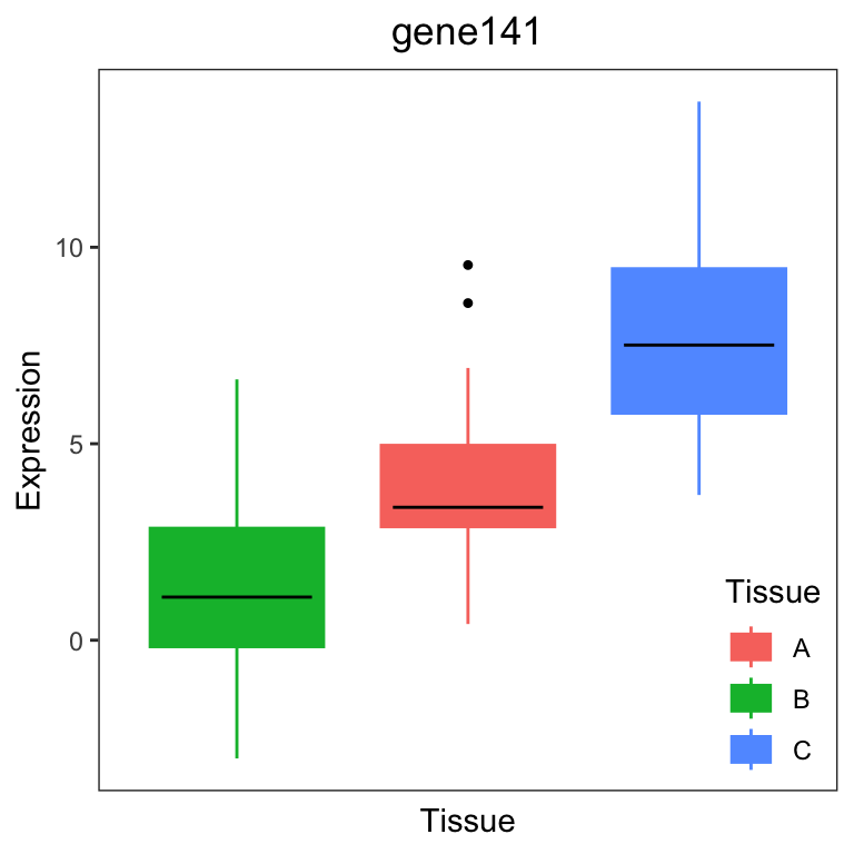

# get gene with the highest variation across Individuals
# create data.frame with expression of gene i and Tissue
#       type for each sample
i <- which.max(varPart$Individual)
GE <- data.frame(
  Expression = geneExpr[i, ],
  Individual = info$Individual
)

# Figure 2b
# plot expression stratified by Tissue
label <- paste("Individual:", format(varPart$Individual[i] * 100,
  digits = 3
), "%")
main <- rownames(geneExpr)[i]
plotStratify(Expression ~ Individual, GE,
  colorBy = NULL,
  text = label, main = main
)

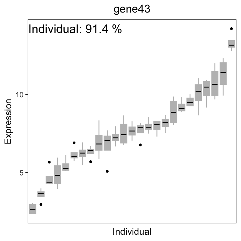
For gene141, variation across tissues explains 52.9% of variance in gene expression. For gene43, variation across Individuals explains 91.4% of variance in gene expression.

Intuition about the backend

At the heart of variancePartition, a regression model is fit for each gene separately and summary statistics are extracted and reported to the user for visualization and downstream analysis. For a single model fit, calcVarPart() computes the fraction of variance explained by each variable. calcVarPart() is defined by this package, and computes these statistics from either a fixed effects model fit with lm() or a linear mixed model fit with lme4::lmer(). fitExtractVarPartModel() loops over each gene, fits the regression model and returns the variance fractions reported by calcVarPart().

Fitting the regression model and extracting variance statistics can also be done directly:

library("lme4")

# fit regression model for the first gene
form_test <- geneExpr[1, ] ~ Age + (1 | Individual) + (1 | Tissue)
fit <- lmer(form_test, info, REML = FALSE)

# extract variance statistics
calcVarPart(fit)

##   Individual       Tissue          Age    Residuals 
## 8.903140e-01 2.468013e-02 4.354738e-05 8.496235e-02

Interpretation

variancePartition fits a linear (mixed) model that jointly considers the contribution of all specified variables on the expression of each gene. It uses a multiple regression model so that the effect of each variable is assessed while jointly accounting for all others. Standard ANOVA implemented in R involves refitting the model while dropping terms, but is aimed at hypothesis testing. calcVarPart() is aimed at estimating variance fractions. It uses a single fit of the linear (mixed) model and evaluates the sum of squares of each term and the sum of squares of the total model fit. However, we note that like any multiple regression model, high correlation bewtween fixed or random effect variables (see Assess correlation between all pairs of variables) can produce unstable estimates and it can be challanging to identify which variable is responsible for the expression variation.

The results of variancePartition give insight into the expression data at multiple levels. Moreover, a single statistic often has multiple equivalent interpretations while only one is relevant to the biological question. Analysis of the example data in Figure 1 gives some strong interpretations.

Considering the median across all genes,

1. variation across individuals explains a median of 81.5% of the variation in expression, after correcting for tissue, batch and age
2. variation across tissues explains a median of 8.2% of the variation in expression, after correcting for other the variables
3. variation across batches is negligible after correcting for variation due to other variables
4. the effect of age is negligible after correcting for other variables
5. correcting for individual, tissue, batch and age leaves a median of 9.3% of the total variance in expression.

These statistics also have a natural interpretation in terms of the intra-class correlation (ICC), the correlation between observations made from samples in the same group.

Considering the median across across all genes and all experiments,

1. the ICC for individual is 81.5%.
2. the ICC for tissue is 8.2%.
3. two randomly selected gene measurements from same individual, but regardless of tissue, batch or age, have a correlation of 81.5%.
4. two randomly selected gene measurements from same tissue, but regardless of individual, batch or age, have a correlation of 8.2%.
5. two randomly selected gene measurements from the same individual and same tissue, but regardless of batch and age, have an correlation of 81.5% + 8.2% = 89.7%.

Note that that the ICC here is interpreted as the ICC after correcting for all other variables in the model.

These conclusions are based on the genome-wide median across all genes, but the same type of statements can be made at the gene-level. Moreover, care must be taken in the interpretation of nested variables. For example, Age is nested within Individual since the multiple samples from each individual are taken at the same age. Thus the effect of Age removes some variation from being explained by Individual. This often arises when considering variation across individuals and across sexes: any cross-sex variation is a component of the cross-individual variation. So the total variation across individuals is the sum of the fraction of variance explained by Sex and Individual. This nesting/summing of effects is common for variables that are properties of the individual rather than the sample. For example, sex and ethnicity are always properties of the individual. Variables like age and disease state can be properties of the individual, but could also vary in time-course or longitudinal experiments. The the interpretation depends on the experimental design.

The real power of variancePartition is to identify specific genes that follow or deviate from the genome-wide trend. The gene-level statistics can be used to identify a subset of genes that are enriched for specific biological functions. For example, we can ask if the 500 genes with the highest variation in expression across tissues (i.e. the long tail for tissue in Figure 1a) are enriched for genes known to have high tissue-specificity.

Should a variable be modeled as fixed or random effect?

Categorical variables should (almost) always be modeled as a random effect. The difference between modeling a categorical variable as a fixed versus random effect is minimal when the sample size is large compared to the number of categories (i.e. levels). So variables like disease status, sex or time point will not be sensitive to modeling as a fixed versus random effect. However, variables with many categories like Individual must be modeled as a random effect in order to obtain statistically valid results. So to be on the safe side, categorical variable should be modeled as a random effect.

% R and variancePartition handle catagorical variables stored as a very naturally. If categorical variables are stored as an or , they must be converted to a before being used with variancePartition

variancePartition fits two types of models:

1. linear mixed model where all categorical variables are modeled as random effects and all continuous variables are fixed effects. The function lme4::lmer() is used to fit this model.

2. fixed effected model, where all variables are modeled as fixed effects. The function lm() is used to fit this model.

Which variables should be included?

In my experience, it is useful to include all variables in the first analysis and then drop variables that have minimal effect. However, like all multiple regression methods, variancePartition will divide the contribution over multiple variables that are strongly correlated. So, for example, including both sex and height in the model will show sex having a smaller contribution to variation gene expression than if height were omitted, since there variables are strongly correlated. This is a simple example, but should give some intuition about a common issue that arises in analyses with variancePartition.

variancePartition can naturally assess the contribution of both individual and sex in a dataset. As expected, genes for which sex explains a large fraction of variation are located on chrX and chrY. If the goal is to interpret the impact of sex, then there is no issue. But recall the issue with correlated variables and note that individual is correlated with sex, because each individual is only one sex regardless of how many samples are taken from a individual. It follows that including sex in the model reduces the apparent contribution of individual to gene expression. In other words, the ICC for individual will be different if sex is included in the model.

In general, including variables in the model that do not vary within individual will reduce the apparent contribution of individual as estimated by variancePartition. For example, sex and ethnicity never vary between multiple samples from the same individual and will always reduce the apparent contribution of individual. However, disease state and age may or may not vary depending on the study design.

In biological datasets technical variability (i.e. batch effects) can often reduce the apparent biological signal. In RNA-seq analysis, it is common for the the impact of this technical variability to be removed before downstream analysis. Instead of including these batch variable in the variancePartition analysis, it is simple to complete the expression residuals with the batch effects removed and then feeds these residuals to variancePartition. This will increase the fraction of variation explained by biological variables since technical variability is reduced.

Assess correlation between all pairs of variables

Evaluating the correlation between variables in a important part in interpreting variancePartition results. When comparing two continuous variables, Pearson correlation is widely used. But variancePartition includes categorical variables in the model as well. In order to accommodate the correlation between a continuous and a categorical variable, or two categorical variables we used canonical correlation analysis.

Canonical Correlation Analysis (CCA) is similar to correlation between two vectors, except that CCA can accommodate matricies as well. For a pair of variables, canCorPairs() assesses the degree to which they co-vary and contain the same information. Variables in the formula can be a continuous variable or a discrete variable expanded to a matrix (which is done in the backend of a regression model). For a pair of variables, canCorPairs() uses CCA to compute the correlation between these variables and returns the pairwise correlation matrix.

Statistically, let rho be the array of correlation values returned by the standard R function cancor to compute CCA. canCorPairs() returns rho / sum(rho) which is the fraction of the maximum possible correlation. Note that CCA returns correlations values between 0 and 1

form <- ~ Individual + Tissue + Batch + Age + Height

# Compute Canonical Correlation Analysis (CCA)
# between all pairs of variables
# returns absolute correlation value
C <- canCorPairs(form, info)

# Plot correlation matrix
# between all pairs of variables
plotCorrMatrix(C)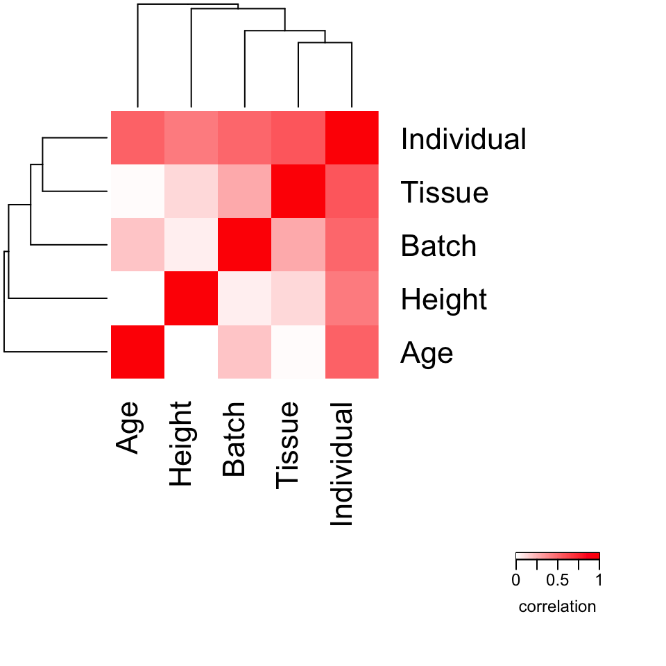

Advanced analysis

Extracting additional information from model fits

Advanced users may want to perform the model fit and extract results in separate steps in order to examine the fit of the model for each gene. Thus the work of can be divided into two steps: 1) fit the regression model, and 2) extracting variance statistics.

form <- ~ Age + (1 | Individual) + (1 | Tissue) + (1 | Batch)

# Fit model
results <- fitVarPartModel(geneExpr, form, info)

# Extract results
varPart <- extractVarPart(results)

Note that storing the model fits can use a lot of memory (~10Gb with 20K genes and 1000 experiments). I do not recommend unless you have a specific need for storing the entire model fit.

Instead, fitVarPartModel() can extract any desired information using any function that accepts the model fit from lm() or lmer(). The results are stored in a list and can be used for downstream analysis.

# Fit model and run summary() function on each model fit
vpSummaries <- fitVarPartModel(geneExpr, form, info, fxn = summary)

# Show results of summary() for the first gene
vpSummaries[[1]]

## Linear mixed model fit by maximum likelihood  ['lmerMod']
## Formula: y.local ~ Age + (1 | Individual) + (1 | Tissue) + (1 | Batch)
##    Data: data
## Weights: data$w.local
## Control: control
## 
##      AIC      BIC   logLik deviance df.resid 
##    397.2    412.8   -192.6    385.2       94 
## 
## Scaled residuals: 
##      Min       1Q   Median       3Q      Max 
## -2.05797 -0.58651  0.01466  0.66030  1.97077 
## 
## Random effects:
##  Groups     Name        Variance Std.Dev.
##  Individual (Intercept) 10.82275 3.28979 
##  Batch      (Intercept)  0.00192 0.04382 
##  Tissue     (Intercept)  0.30010 0.54781 
##  Residual                1.02997 1.01488 
## Number of obs: 100, groups:  Individual, 25; Batch, 4; Tissue, 3
## 
## Fixed effects:
##               Estimate Std. Error t value
## (Intercept) -10.602426   1.094925  -9.683
## Age           0.003183   0.016103   0.198
## 
## Correlation of Fixed Effects:
##     (Intr)
## Age -0.739

Removing batch effects before fitting model

Gene expression studies often have substantial batch effects, and variancePartition can be used to understand the magnitude of the effects. However, we often want to focus on biological variables (i.e. individual, tissue, disease, sex) after removing the effect of technical variables. Depending on the size of the batch effect, I have found it useful to correct for the batch effect first and then perform a variancePartition analysis afterward. Subtracting this batch effect can reduce the total variation in the data, so that the contribution of other variables become clearer.

Standard analysis:

form <- ~ (1 | Tissue) + (1 | Individual) + (1 | Batch) + Age
varPart <- fitExtractVarPartModel(geneExpr, form, info)

Analysis on residuals:

library("limma")
# subtract out effect of Batch
fit <- lmFit(geneExpr, model.matrix(~Batch, info))
res <- residuals(fit, geneExpr)

# fit model on residuals
form <- ~ (1 | Tissue) + (1 | Individual) + Age

varPartResid <- fitExtractVarPartModel(res, form, info)

Remove batch effect with linear mixed model

# subtract out effect of Batch with linear mixed model
modelFit <- fitVarPartModel(geneExpr, ~ (1 | Batch), info)
res <- residuals(modelFit)

# fit model on residuals
form <- ~ (1 | Tissue) + (1 | Individual) + Age

varPartResid <- fitExtractVarPartModel(res, form, info)

If the two-step process requires too much memory, the residuals can be computed more efficiently. Here, run the function inside the call to fitVarPartModel() to avoid storing the large intermediate results.

# extract residuals directly without storing intermediate results
residList <- fitVarPartModel(geneExpr, ~ (1 | Batch), info,
  fxn = residuals
)

# convert list to matrix
residMatrix <- do.call(rbind, residList)

Variation within multiple subsets of the data

So far, we have focused on interpreting one variable at a time. But the linear mixed model behind variancePartition is a very powerful framework for analyzing variation at multiple levels. We can easily extend the previous analysis of the contribution of individual and tissue on variation in gene expression to examine the contribution of individual within each tissue. This analysis is as easy as specifying a new formula and rerunning variancePartition. Note that is analysis will only work when there are replicates for at least some individuals within each tissue in order to assess cross-individual variance with in a tissue.

# specify formula to model within/between individual variance
# separately for each tissue
# Note that including +0 ensures each tissue is modeled explicitly
# Otherwise, the first tissue would be used as baseline
form <- ~ (Tissue + 0 | Individual) + Age + (1 | Tissue) + (1 | Batch)

# fit model and extract variance percents
varPart <- fitExtractVarPartModel(geneExpr, form, info, showWarnings = FALSE)

# violin plot
plotVarPart(sortCols(varPart), label.angle = 60)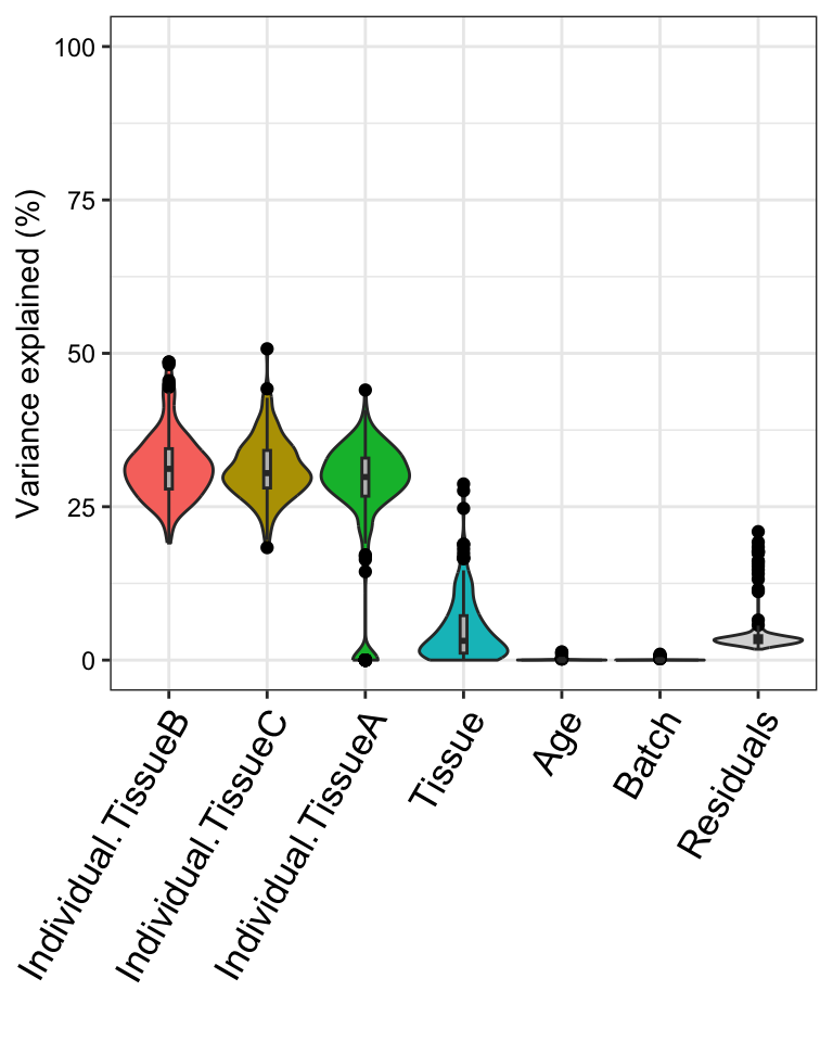

This analysis corresponds to a varying coefficient model, where the correlation between individuals varies for each tissue ]. Since the variation across individuals is modeled within each tissue, the total variation explained does not sum to 1 as it does for standard application of variancePartition. So interpretation as intra-class does not strictly apply and use of plotPercentBars() is no longer applicable. Yet the variables in the study design are still ranked in terms of their genome-wide contribution to expression variation, and results can still be analyzed at the gene level. See Variation with multiple subsets of the data for statistical details.

Detecting problems caused by collinearity of variables

Including variables that are highly correlated can produce misleading results and overestimate the contribution of variables modeled as fixed effects. This is usually not an issue, but can arise when statistically redundant variables are included in the model. In this case, the model is "degenerate" or "computationally singular" and parameter estimates from this model are not meaningful. Dropping one or more of the covariates will fix this problem.

A check of collinearity is built into fitVarPartModel() and fitExtractVarPartModel(), so the user will be warned if this is an issue.

Alternatively, the user can use the colinearityScore() function to evaluate whether this is an issue for a single model fit:

form <- ~ (1 | Individual) + (1 | Tissue) + Age + Height

# fit model
res <- fitVarPartModel(geneExpr[1:4, ], form, info)

# evaluate the collinearity score on the first model fit
# this reports the correlation matrix between coefficient estimates
# for fixed effects
# the collinearity score is the maximum absolute correlation value
# If the collinearity score > .99 then the variance partition
# estimates may be problematic
# In that case, a least one variable should be omitted
colinearityScore(res[[1]])

## [1] 0.7774082
## attr(,"vcor")
##             (Intercept)         Age      Height
## (Intercept)   1.0000000 -0.41907978 -0.77740819
## Age          -0.4190798  1.00000000 -0.05748224
## Height       -0.7774082 -0.05748224  1.00000000

Including weights computed separately

variancePartition automatically used precision weights computed by limma::voom(), but the user can also specify custom weights using the weightsMatrix argument.

form <- ~ (1 | Individual) + (1 | Tissue) + Age + Height

# Specify custom weights
# In this example the weights are simulated from a
# uniform distribution and are not meaningful.
weights <- matrix(runif(length(geneExpr)), nrow = nrow(geneExpr))

# Specify custom weights
res <- fitExtractVarPartModel(geneExpr[1:4, ], form, info,
  weightsMatrix = weights[1:4, ]
)

In addition, setting the useWeights=FALSE will suppress usage of the weights in all cases, i.e. when the weights are specified manually or implicitly with the results of limma::voom().

Including interaction terms

Typical analysis assumes that the effect of each variable on gene expression does not depend on other variables in the model. Sometimes this assumption is too strict, and we want to model an interaction effect whereby the effect of Batch depends on Tissue. This can be done easly by specifying an interaction term, (1|Batch:Tissue). Since Batch has 4 categories and Tissue has 3, this interaction term implicity models a new 3*4 = 12 category variable in the analysis. This new interaction term will absorb some of the variance from the Batch and Tissue term, so an interaction model should always include the two constituent variables.

Here we fit an interaction model, but we observe that interaction between Batch and Tissue does not explain much expression variation.

form <- ~ (1 | Individual) + Age + Height + (1 | Tissue) + (1 | Batch) +
  (1 | Batch:Tissue)

# fit model
vpInteraction <- fitExtractVarPartModel(geneExpr, form, info)

plotVarPart(sortCols(vpInteraction))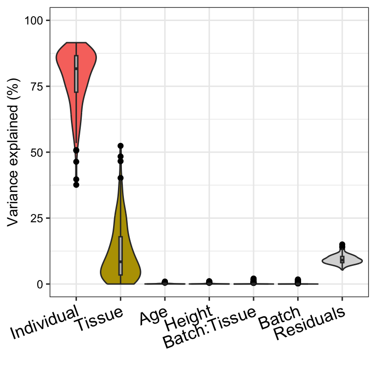

Application to expression data

variancePartition works with gene expression data that has already been processed and normalized as for differential expression analysis.

Gene-level counts

featureCounts (Liao, Smyth, and Shi 2014) and HTSeq (Anders, Pyl, and Huber 2015) report the number of reads mapping to each gene (or exon). These results are easily read into R. limma::voom() and DESeq2 are widely used for differential expression analysis of gene- and exon-level counts and can be used to process data before analysis with variancePartition. This section addresses processing and normalization of gene-level counts, but the analysis is the same for exon-level counts.

limma::voom()

Read RNA-seq counts into R, normalize for library size within and between experiments with TMM (Robinson and Oshlack 2010), estimate precision weights with limma::voom().

library("limma")
library("edgeR")

# identify genes that pass expression cutoff
isexpr <- rowSums(cpm(geneCounts) > 1) >= 0.5 * ncol(geneCounts)

# create data structure with only expressed genes
gExpr <- DGEList(counts = geneCounts[isexpr, ])

# Perform TMM normalization
gExpr <- calcNormFactors(gExpr)

# Specify variables to be included in the voom() estimates of
# uncertainty.
# Recommend including variables with a small number of categories
# that explain a substantial amount of variation
design <- model.matrix(~Batch, info)

# Estimate precision weights for each gene and sample
# This models uncertainty in expression measurements
vobjGenes <- voom(gExpr, design)

# Define formula
form <- ~ (1 | Individual) + (1 | Tissue) + (1 | Batch) + Age

# variancePartition seamlessly deals with the result of voom()
# by default, it seamlessly models the precision weights
# This can be turned off with useWeights=FALSE
varPart <- fitExtractVarPartModel(vobjGenes, form, info)

DESeq2

Process and normalize the gene-level counts before running variancePartition analysis.

library("DESeq2")

# create DESeq2 object from gene-level counts and metadata
dds <- DESeqDataSetFromMatrix(
  countData = geneCounts,
  colData = info,
  design = ~1
)

# Estimate library size correction scaling factors
dds <- estimateSizeFactors(dds)

# identify genes that pass expression cutoff
isexpr <- rowSums(fpm(dds) > 1) >= 0.5 * ncol(dds)

# compute log2 Fragments Per Million
# Alternatively, fpkm(), vst() or rlog() could be used
quantLog <- log2(fpm(dds)[isexpr, ] + 1)

# Define formula
form <- ~ (1 | Individual) + (1 | Tissue) + (1 | Batch) + Age

# Run variancePartition analysis
varPart <- fitExtractVarPartModel(quantLog, form, info)

Note that DESeq2 does not compute precision weights like limma::voom(), so they are not used in this version of the analysis.

Isoform quantification

Other software performs isoform-level quantification using reads that map to multiple transcripts. These include kallisto (Bray et al. 2016), sailfish (Patro, Mount, and Kingsford 2014), salmon Patro, Duggal, and Kingsford (2015), RSEM (Li and Dewey 2011 )and cufflinks (Trapnell et al. 2010.)

tximport

Quantifications from kallisto, salmon, sailfish and RSEM can be read into R and processed with the Bioconductor package tximport. The gene- or transcript-level quantifications can be used directly in variancePartition.

library("tximportData")
library("tximport")
library("readr")

# Get data from folder where tximportData is installed
dir <- system.file("extdata", package = "tximportData")
samples <- read.table(file.path(dir, "samples.txt"), header = TRUE)
files <- file.path(dir, "kallisto", samples$run, "abundance.tsv")
names(files) <- paste0("sample", 1:6)

tx2gene <- read.csv(file.path(dir, "tx2gene.csv"))

# reads results from kallisto
txi <- tximport(files,
  type = "kallisto", tx2gene = tx2gene,
  countsFromAbundance = "lengthScaledTPM"
)

# define metadata (usually read from external source)
info_tximport <- data.frame(
  Sample = sprintf("sample%d", 1:6),
  Disease = c("case", "control")[c(rep(1, 3), rep(2, 3))]
)

# Extract counts from kallisto
y <- DGEList(txi$counts)

# compute library size normalization
y <- calcNormFactors(y)

# apply voom to estimate precision weights
design <- model.matrix(~Disease, data = info_tximport)
vobj <- voom(y, design)

# define formula
form <- ~ (1 | Disease)

# Run variancePartition analysis (on only 10 genes)
varPart_tx <- fitExtractVarPartModel(
  vobj[1:10, ], form,
  info_tximport
)

Code to process results from sailfish, salmon, RSEM is very similar.

See tutorial for more details.

ballgown

Quantifications from Cufflinks/Tablemaker and RSEM can be processed and read into R with the Bioconductor package ballgown.

library("ballgown")

# Get data from folder where ballgown is installed
data_directory <- system.file("extdata", package = "ballgown")

# Load results of Cufflinks/Tablemaker
bg <- ballgown(
  dataDir = data_directory, samplePattern = "sample",
  meas = "all"
)

# extract gene-level FPKM quantification
# Expression can be convert to log2-scale if desired
gene_expression <- gexpr(bg)

# extract transcript-level FPKM quantification
# Expression can be convert to log2-scale if desired
transcript_fpkm <- texpr(bg, "FPKM")

# define metadata (usually read from external source)
info_ballgown <- data.frame(
  Sample = sprintf("sample%02d", 1:20),
  Batch = rep(letters[1:4], 5),
  Disease = c("case", "control")[c(rep(1, 10), rep(2, 10))]
)

# define formula
form <- ~ (1 | Batch) + (1 | Disease)

# Run variancePartition analysis
# Gene-level analysis
varPart_gene <- fitExtractVarPartModel(
  gene_expression, form,
  info_ballgown
)

## Warning in filterInputData(exprObj, formula, data, useWeights = useWeights): Sample names of responses (i.e. columns of exprObj) do not match
## sample names of metadata (i.e. rows of data).  Recommend consistent
## names so downstream results are labeled consistently.

## Warning in .fitExtractVarPartModel(exprObj, formula, data, REML = REML, : Model failed for 1 responses.
##   See errors with attr(., 'errors')

# Transcript-level analysis
varPart_transcript <- fitExtractVarPartModel(
  transcript_fpkm, form,
  info_ballgown
)

## Warning in filterInputData(exprObj, formula, data, useWeights = useWeights): Sample names of responses (i.e. columns of exprObj) do not match
## sample names of metadata (i.e. rows of data).  Recommend consistent
## names so downstream results are labeled consistently.

## Warning in .fitExtractVarPartModel(exprObj, formula, data, REML = REML, : Model failed for 2 responses.
##   See errors with attr(., 'errors')

Note that ballgownrsem can be used for a similar analysis of RSEM results.

See tutorial for more details.

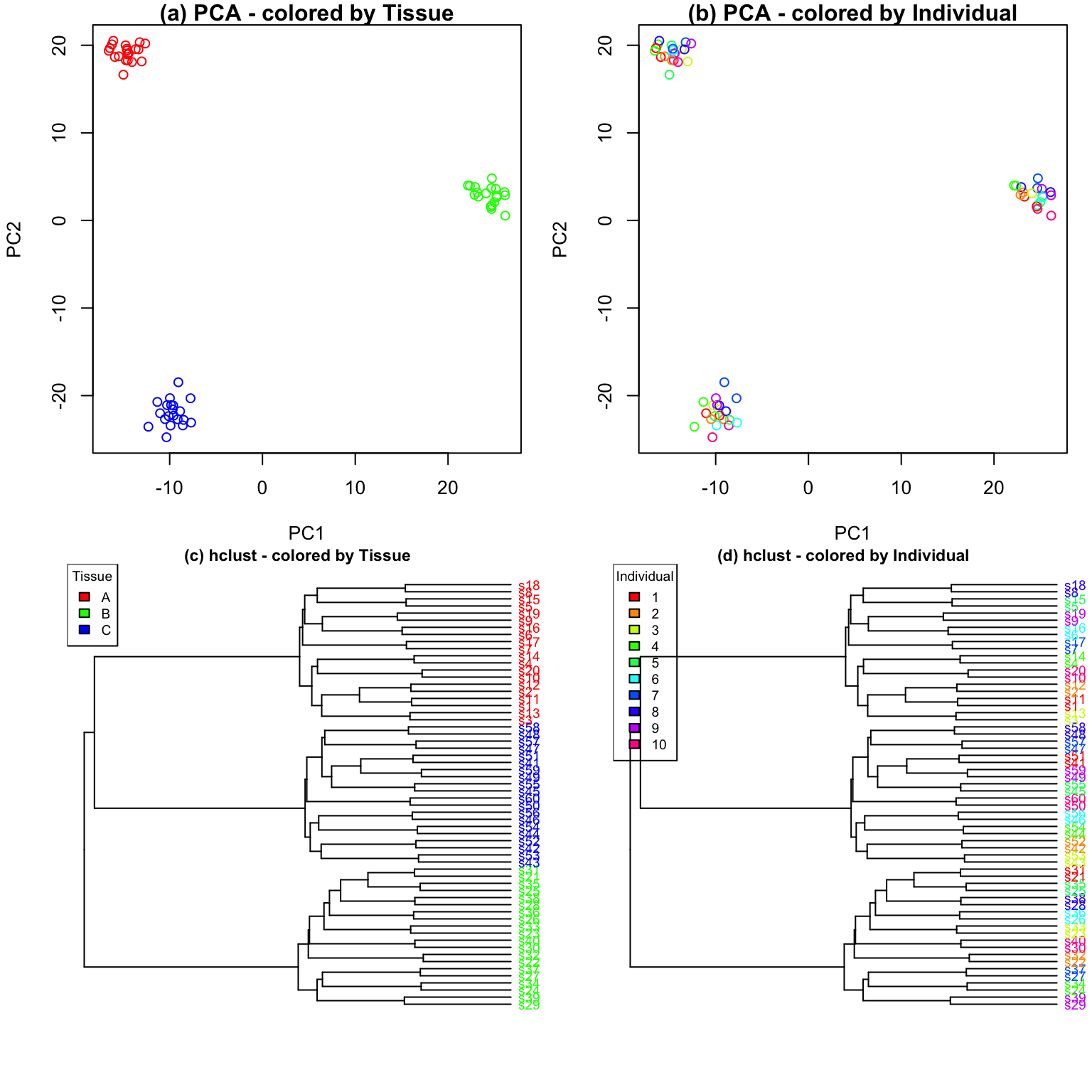
Compare with other methods

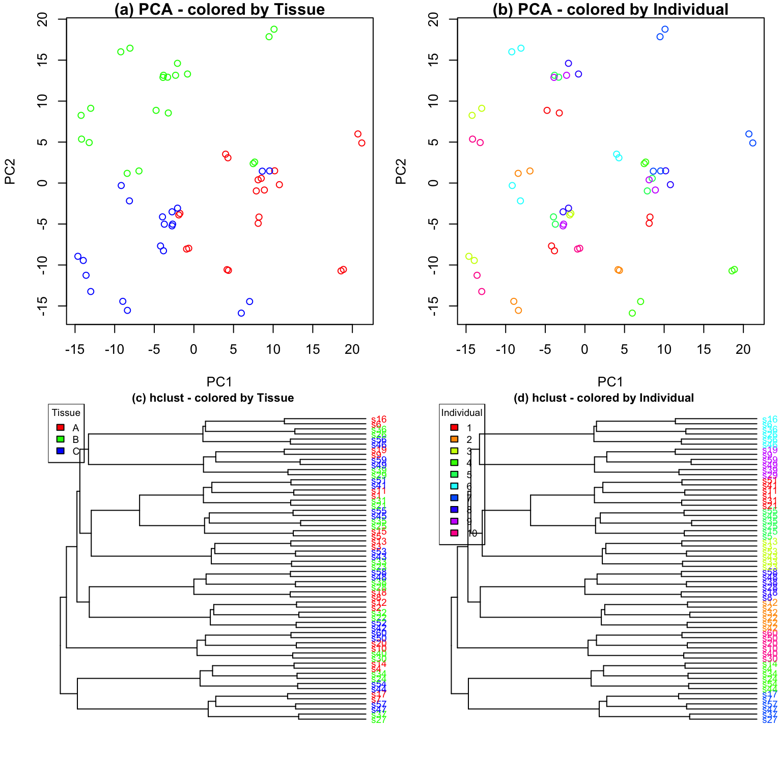
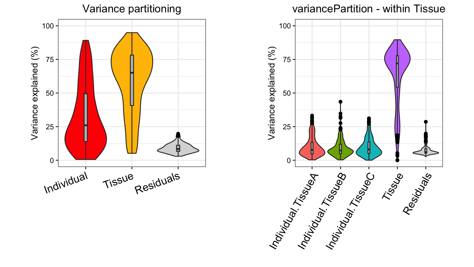
Characterizing drivers of variation in gene expression data has typically relied on principal components analysis (PCA) and hierarchical clustering. Here I apply these methods to two simulated datasets to demonstrate the additional insight from an analysis with variancePartition. Each simulated dataset comprises 60 experiments from 10 individuals and 3 tissues with 2 biological replicates. In the first dataset, tissue is the major driver of variation in gene expression(Figure @ref(fig:siteDominant)). 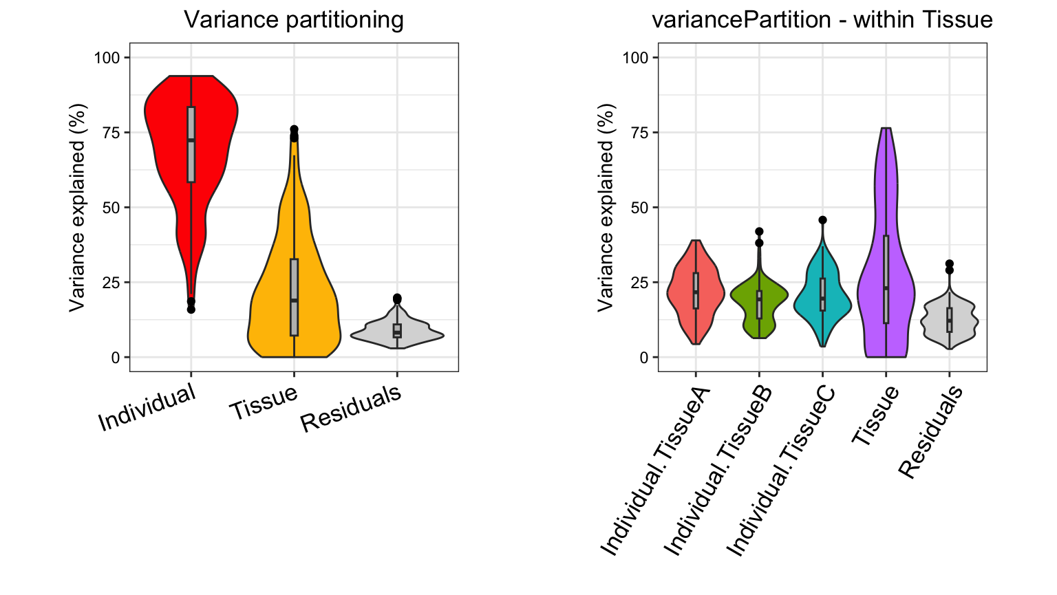In the second dataset, individual is the major driver of variation in gene expression (Figures @ref(fig:IndivDominant)).

Analysis of simulated data illustrates that PCA identifies the major driver of variation when tissue is dominant and there are only 3 categories. But the results are less clear when individual is dominant because there are now 10 categories. Meanwhile, hierarchical clustering identifies the major driver of variation in both cases, but does not give insight into the second leading contributor.

Analysis with variancePartition has a number of advantages over these standard methods:

1. variancePartition provides a natural interpretation of multiple variables

   • figures from PCA/hierarchical clustering allow easy interpretation of only one variable

2. variancePartition quantifies the contribution of each variable

   • PCA/hierarchical clustering give only a visual representation

3. variancePartition interprets contribution of each variable to each gene individually for downstream analysis

   • PCA/hierarchical clustering produces genome-wide summary and does not allow gene-level interpretation

4. variancePartition can assess contribution of one variable (i.e. Individual) separately in subset of the data defined by another variable (i.e. Tissue)

Tissue is major source of variation

Individual is major source of variation

Statistical details

A variancePartition analysis evaluates the linear (mixed) model \[\begin{eqnarray} y &=& \sum_j X_j\beta_j + \sum_k Z_k \alpha_k + \varepsilon \\ \alpha_k &\sim& \mathcal{N}(0, \sigma^2_{\alpha_k})\\ \varepsilon &\sim& \mathcal{N}(0, \sigma^2_\varepsilon) \end{eqnarray}\] where \(y\) is the expression of a single gene across all samples, \(X_j\) is the matrix of \(j^{th}\) fixed effect with coefficients \(\beta_j\), \(Z_k\) is the matrix corresponding to the \(k^{th}\) random effect with coefficients \(\alpha_k\) drawn from a normal distribution with variance \(\sigma^2_{\alpha_k}\). The noise term, \(\varepsilon\), is drawn from a normal distribution with variance \(\sigma^2_\varepsilon\). Parameters are estimated with maximum likelihood, rather than REML, so that fixed effect coefficients, \(\beta_j\), are explicitly estimated.

I use the term “linear (mixed) model” here since variancePartition works seamlessly when a fixed effects model (i.e. linear model) is specified.

Variance terms for the fixed effects are computed using the post hoc calculation
\[\begin{eqnarray} \hat{\sigma}^2_{\beta_j} = \text{var}\left( X_j \hat{\beta}_j\right). \end{eqnarray}\] For a fixed effects model, this corresponds to the sum of squares for each component of the model.

For a standard application of the linear mixed model, where the effect of each variable is additive, the fraction of variance explained by the \(j^{th}\) fixed effect is \[\begin{eqnarray} \frac{\hat{\sigma}^2_{\beta_j}}{\sum_j \hat{\sigma}^2_{\beta_j} + \sum_k \hat{\sigma}^2_{\alpha_k} + \hat{\sigma}^2_\varepsilon}, \end{eqnarray}\] by the \(k^{th}\) random effect is \[\begin{eqnarray} \frac{\hat{\sigma}^2_{\alpha_k}}{\sum_j \hat{\sigma}^2_{\beta_j} + \sum_k \hat{\sigma}^2_{\alpha_k} + \hat{\sigma}^2_\varepsilon}, \end{eqnarray}\] and the residual variance is \[\begin{eqnarray} \frac{\hat{\sigma}^2_{\varepsilon}}{\sum_j \hat{\sigma}^2_{\beta_j} + \sum_k \hat{\sigma}^2_{\alpha_k} + \hat{\sigma}^2_\varepsilon}. \end{eqnarray}\]

Implementation in R

An R formula is used to define the terms in the fixed and random effects, and fitVarPartModel() fits the specified model for each gene separately. If random effects are specified, lme4::lmer() is used behind the scenes to fit the model, while lm() is used if there are only fixed effects. fitVarPartModel() returns a list of the model fits, and returns the variance partition statistics for each model in the list. fitExtractVarPartModel() combines the actions of fitVarPartModel() and into one function call. calcVarPart() is called behind the scenes to compute variance fractions for both fixed and mixed effects models, but the user can also call this function directly on a model fit with lm() or lmer().

Interpretation of percent variance explained

The percent variance explained can be interpreted as the intra-class correlation (ICC) when a special case of Equation 1 is used. Consider the simplest example of the \(i^{th}\) sample from the \(k^{th}\) individual \[\begin{eqnarray} y_{i,k} = \mu + Z \alpha_{i,k} + e_{i,k} \end{eqnarray}\] with only an intercept term, one random effect corresponding to individual, and an error term. In this case ICC corresponds to the correlation between two samples from the same individual. This value is equal to the fraction of variance explained by individual. For example, consider the correlation between samples from the same individual: \[\begin{eqnarray} ICC &=& cor( y_{1,k}, y_{2,k}) \\ &=& cor( \mu + Z \alpha_{1,k} + e_{1,k}, \mu + Z \alpha_{2,k} + e_{2,k}) \\ &=& \frac{cov( \mu + Z \alpha_{1,k} + e_{1,k}, \mu + Z \alpha_{2,k} + e_{2,k})}{ \sqrt{ var(\mu + Z \alpha_{1,k} + e_{1,k}) var( \mu + Z \alpha_{2,k} + e_{2,k})}}\\ &=& \frac{cov(Z \alpha_{1,k}, Z \alpha_{2,k})}{\sigma^2_\alpha + \sigma^2_\varepsilon} \\ &=& \frac{\sigma^2_\alpha}{\sigma^2_\alpha + \sigma^2_\varepsilon} \end{eqnarray}\] The correlation between samples from different individuals is: \[\begin{eqnarray} &=& cor( y_{1,1}, y_{1,2}) \\ &=& cor( \mu + Z \alpha_{1,1} + e_{1,1}, \mu + Z \alpha_{1,2} + e_{1,2}) \\ &=& \frac{cov(Z \alpha_{1,1}, Z \alpha_{1,2})}{\sigma^2_\alpha + \sigma^2_\varepsilon} \\ &=& \frac{0}{\sigma^2_\alpha + \sigma^2_\varepsilon} \\ &=& 0 \end{eqnarray}\] This interpretation in terms of fraction of variation explained (FVE) naturally generalizes to multiple variance components. Consider two sources of variation, individual and cell type with variances \(\sigma^2_{id}\) and \(\sigma^2_{cell},\) respectively. Applying a generalization of the the previous derivation, two samples are correlated according to:

Individual	cell type	variance	Interpretation	Correlation value
same	different	\(\frac{\sigma^2_{id}}{\sigma^2_{id} + \sigma^2_{cell} + \sigma^2_\varepsilon }\)	FVE by individual	\(ICC_{individual}\)
different	same	\(\frac{\sigma^2_{cell}}{\sigma^2_{id} + \sigma^2_{cell} + \sigma^2_\varepsilon }\)	FVE by cell type	\(ICC_{cell}\)
same	same	\(\frac{\sigma^2_{id} + \sigma^2_{cell}}{\sigma^2_{id} + \sigma^2_{cell} + \sigma^2_\varepsilon }\)	sum of FVE by individual & cell type	\(ICC_{individual,cell}\)
different	different	\(\frac{0}{\sigma^2_{id} + \sigma^2_{cell} + \sigma^2_\varepsilon }\)	sample are independent

Notice that the correlation between samples from the same individual and same cell type corresponds to the sum of the fraction explained by individual + fraction explained by cell type. This defines ICC for individual and tissue, as well as the combined ICC and relates these values to FVE.

In order to illustrate how this FVE and ICC relate to the correlation between samples in multilevel datasets, consider a simple example of 5 samples from 2 individuals and 2 tissues:

Sample	Individual	Cell type
a	1	T-Cell
b	1	T-Cell
c	1	monocyte
d	2	T-Cell
e	2	monocyte

Modeling the separate effects of individual and tissue gives the following covariance structure between samples when a linear mixed model is used:

\[ \begin{array}{ccc} & \\ cov(y)=\begin{array}{ccccc} a \\ b \\ c\\ d\\ e\end{array} & \left( \begin{array}{ccccc} \sigma^2_{id} + \sigma^2_{cell} + \sigma^2_\varepsilon & & &&\\ \sigma^2_{id} + \sigma^2_{cell} & \sigma^2_{id} + \sigma^2_{cell} + \sigma^2_\varepsilon & & &\\ \sigma^2_{id} & \sigma^2_{id} &\sigma^2_{id} + \sigma^2_{cell} + \sigma^2_\varepsilon & &\\ \sigma^2_{cell} & \sigma^2_{cell} &0 &\sigma^2_{id} + \sigma^2_{cell} + \sigma^2_\varepsilon &\\ 0 & 0 &\sigma^2_{cell} & \sigma^2_{id} &\sigma^2_{id} + \sigma^2_{cell} + \sigma^2_\varepsilon \\ \end{array} \right)\end{array} \]

The covariance matrix is symmetric so that blank entries take the value on the opposite side of the diagonal. The covariance can be converted to correlation by dividing by \(\sigma^2_{id} + \sigma^2_{cell} + \sigma^2_\varepsilon\), and this gives the results from above. This example generalizes to any number of variance components (Pinheiro and Bates 2000).

Variation with multiple subsets of the data

The linear mixed model underlying variancePartition allows the effect of one variable to depend on the value of another variable. Statistically, this is called a varying coefficient model (Pinheiro and Bates 2000; Galecki and Burzykowski 2013). This model arises in variancePartition analysis when the variation explained by individual depends on tissue or cell type.

A given sample is only from one cell type, so this analysis asks a question about a subset of the data. The the data is implicitly divided into subsets base on cell type and variation explained by individual is evaluated within each subset. The data is not actually divided onto subset, but the statistical model essentially examples samples with each cell type. This subsetting means that the variance fractions do not sum to 1.

Consider a concrete example with variation from across individual and cell types (T-cells and monocytes) with data from the \(i^{th}\) sample from the \(k^{th}\) individual, sex of \(s\) and cell type \(c\). Modeling the variation across individuals within cell type corresponds to \[\begin{eqnarray} y_{i,k,s,c} = \mu + Z^{(sex)} \alpha_{i,s} + Z^{(Tcell| id)} \alpha_{i,k,c} + Z^{(monocyte| id)} \alpha_{i,k,c} + e_{i,k,s,c} \end{eqnarray}\]

with corresponding variance components:

Variance component	Interpretation
\(\sigma^2_{sex}\)	variance across sex (which is the same for all cell types)
\(\sigma^2_{(Tcell| id)}\)	variance across individuals within T-cells
\(\sigma^2_{(monocyte| id)}\)	variance across individuals within monocytes
\(\sigma^2_\varepsilon\)	residual variance

Since the dataset is now divided into multiple subsets, direct interpretation of the fraction of variation explained (FVE) as intra-class correlation does not apply. Instead, we compute a “pseudo-FVE” by approximating the total variance attributable to cell type by using a weighted average of the within cell type variances weighted by the sample size within each cell type. Thus the values of pseudo-FVE do not have the simple interpretation as in the standard application of variancePartition, but allows ranking of variables based on genome-wide contribution to variance and analysis of gene-level results.

Variance partitioning and differential expression

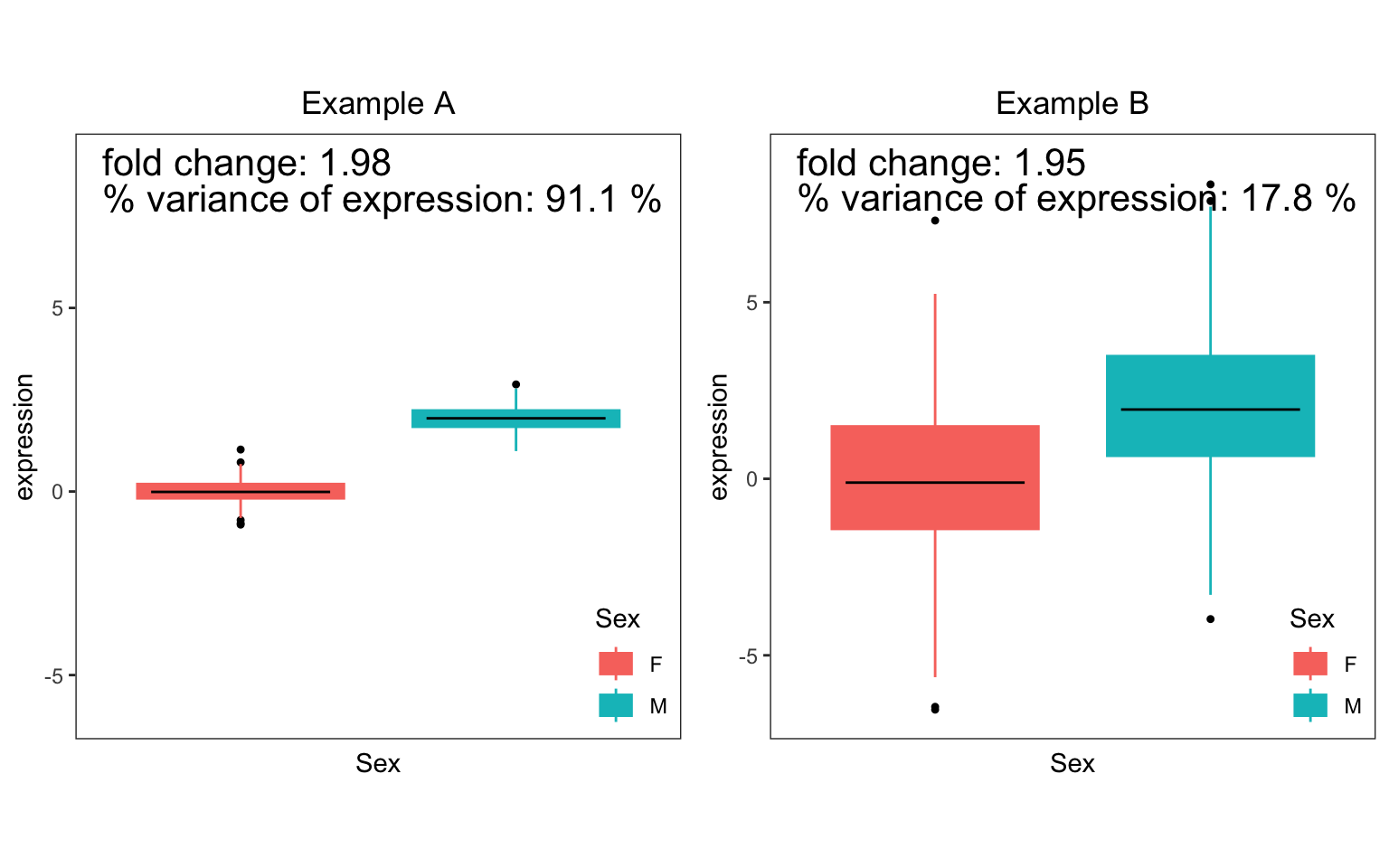
Differential expression (DE) is widely used to identify gene which show difference is expression between two subsets of the data (i.e. case versus controls). For a single gene, DE analysis measures the difference in mean expression between the two subsets. (Since expression is usually analyzed on a log scale, DE results are usually shown in terms of log fold changes between the two subsets ). In the Figure, consider two simulated examples of a gene whose expression differs between males and females. The mean expression in males is 0 and the mean expression in females is 2 in both cases. Therefore, the fold change is 2 in both cases.

However, the fraction of expression variation explained by sex is very different in these two examples. In example A, there is very little variation within each sex, so that variation between sexes is very high at 91.1%. Conversely, example B shows high variation within sexes, so that variation between sexes is only 17.8%.

The fact that the fold change or the fraction of variation is significantly different from 0 indicates differential expression between the two sexes. Yet these two statistics have different interpretations. The fold change from DE analysis tests a difference in means between two sexes. The fraction of variation explained compares the variation explained by sex to the total variation.

Thus the fraction of variation explained reported by variancePartition reflects as different aspect of the data not captured by DE analysis.

Modelling error in gene expression measurements

Uncertainty in the measurement of gene expression can be modeled with precision weights and tests of differentially expression using limma::voom() model this uncertainty directly with a heteroskedastic linear regression (Law et al. 2014). variancePartition can use these precision weights in a heteroskedastic linear mixed model implemented in lme4 (Bates et al. 2015). These precision weights are used seamlessly by calling fitVarPartModel() or fitExtractVarPartModel() on the output of limma::voom(). Otherwise the user can specify the weights with the weightsMatrix parameter.

Session Info

## R version 4.3.0 (2023-04-21)
## Platform: x86_64-apple-darwin22.4.0 (64-bit)
## Running under: macOS 14.2.1
## 
## Matrix products: default
## BLAS:   /Users/gabrielhoffman/prog/R-4.3.0/lib/libRblas.dylib 
## LAPACK: /usr/local/Cellar/r/4.3.0_1/lib/R/lib/libRlapack.dylib;  LAPACK version 3.11.0
## 
## locale:
## [1] en_US.UTF-8/en_US.UTF-8/en_US.UTF-8/C/en_US.UTF-8/en_US.UTF-8
## 
## time zone: America/New_York
## tzcode source: internal
## 
## attached base packages:
## [1] stats4    stats     graphics  grDevices utils     datasets  methods   base     
## 
## other attached packages:
##  [1] dendextend_1.17.1           ballgown_2.32.0             DESeq2_1.40.1              
##  [4] SummarizedExperiment_1.30.1 Biobase_2.60.0              MatrixGenerics_1.12.0      
##  [7] matrixStats_1.0.0           GenomicRanges_1.52.0        GenomeInfoDb_1.36.1        
## [10] IRanges_2.34.1              S4Vectors_0.38.1            BiocGenerics_0.46.0        
## [13] edgeR_3.42.4                lme4_1.1-34                 Matrix_1.5-4.1             
## [16] variancePartition_1.33.11   BiocParallel_1.34.2         limma_3.56.2               
## [19] ggplot2_3.4.4              
## 
## loaded via a namespace (and not attached):
##   [1] RColorBrewer_1.1-3       jsonlite_1.8.5           magrittr_2.0.3          
##   [4] farver_2.1.1             nloptr_2.0.3             rmarkdown_2.22          
##   [7] fs_1.6.2                 BiocIO_1.10.0            zlibbioc_1.46.0         
##  [10] ragg_1.2.5               vctrs_0.6.3              memoise_2.0.1           
##  [13] minqa_1.2.5              Rsamtools_2.16.0         RCurl_1.98-1.12         
##  [16] htmltools_0.5.5          S4Arrays_1.2.0           broom_1.0.5             
##  [19] sass_0.4.6               KernSmooth_2.23-21       bslib_0.4.2             
##  [22] desc_1.4.2               pbkrtest_0.5.2           plyr_1.8.8              
##  [25] cachem_1.0.8             GenomicAlignments_1.36.0 lifecycle_1.0.3         
##  [28] iterators_1.0.14         pkgconfig_2.0.3          R6_2.5.1                
##  [31] fastmap_1.1.1            GenomeInfoDbData_1.2.10  rbibutils_2.2.13        
##  [34] digest_0.6.33            numDeriv_2016.8-1.1      colorspace_2.1-0        
##  [37] AnnotationDbi_1.62.1     rprojroot_2.0.3          textshaping_0.3.6       
##  [40] RSQLite_2.3.1            labeling_0.4.2           fansi_1.0.4             
##  [43] mgcv_1.8-42              httr_1.4.6               abind_1.4-5             
##  [46] compiler_4.3.0           bit64_4.0.5              aod_1.3.2               
##  [49] withr_2.5.0              backports_1.4.1          viridis_0.6.3           
##  [52] DBI_1.1.3                highr_0.10               gplots_3.1.3            
##  [55] MASS_7.3-60              DelayedArray_0.26.3      rjson_0.2.21            
##  [58] corpcor_1.6.10           gtools_3.9.4             caTools_1.18.2          
##  [61] tools_4.3.0              remaCor_0.0.17           glue_1.6.2              
##  [64] restfulr_0.0.15          nlme_3.1-162             grid_4.3.0              
##  [67] reshape2_1.4.4           generics_0.1.3           sva_3.48.0              
##  [70] gtable_0.3.3             tidyr_1.3.0              utf8_1.2.3              
##  [73] XVector_0.40.0           pillar_1.9.0             stringr_1.5.0           
##  [76] genefilter_1.82.1        splines_4.3.0            dplyr_1.1.2             
##  [79] lattice_0.21-8           survival_3.5-5           rtracklayer_1.60.0      
##  [82] bit_4.0.5                annotate_1.78.0          tidyselect_1.2.0        
##  [85] locfit_1.5-9.7           Biostrings_2.68.1        knitr_1.43              
##  [88] gridExtra_2.3            RhpcBLASctl_0.23-42      xfun_0.39               
##  [91] stringi_1.7.12           yaml_2.3.7               boot_1.3-28.1           
##  [94] evaluate_0.21            codetools_0.2-19         tibble_3.2.1            
##  [97] cli_3.6.1                xtable_1.8-4             systemfonts_1.0.4       
## [100] Rdpack_2.4               munsell_0.5.0            jquerylib_0.1.4         
## [103] Rcpp_1.0.11              EnvStats_2.7.0           png_0.1-8               
## [106] XML_3.99-0.14            parallel_4.3.0           pkgdown_2.0.7           
## [109] blob_1.2.4               bitops_1.0-7             viridisLite_0.4.2       
## [112] mvtnorm_1.2-2            lmerTest_3.1-3           scales_1.2.1            
## [115] purrr_1.0.2              crayon_1.5.2             fANCOVA_0.6-1           
## [118] rlang_1.1.1              cowplot_1.1.1            KEGGREST_1.40.0

References

Anders, Simon, Paul Theodor Pyl, and Wolfgang Huber. 2015. “HTSeq-A Python framework to work with high-throughput sequencing data.” Bioinformatics 31 (2): 166–69. https://doi.org/10.1093/bioinformatics/btu638.

Bates, D., M. Machler, B. Bolker, and S. Walker. 2015. “Fitting Linear Mixed-Effects Models Using lme4.” Journal of Statistical Software 67 (1). https://doi.org/10.18637/jss.v067.i01.

Bray, Nicolas L, Harold Pimentel, Páll Melsted, and Lior Pachter. 2016. “Near-optimal probabilistic RNA-seq quantification.” Nature Biotechnology 34: 525–27. https://doi.org/10.1038/nbt.3519.

Carvalho, Benilton S, and Rafael A Irizarry. 2010. “A Framework for Oligonucleotide Microarray Preprocessing.” Bioinformatics 26 (19): 2363–67. https://doi.org/10.1093/bioinformatics/btq431.

Frazee, Alyssa C, Geo Pertea, Andrew E Jaffe, Ben Langmead, Steven L Salzberg, and Jeffrey T Leek. 2015. “Ballgown bridges the gap between transcriptome assembly and expression analysis.” Nature Biotechnology 33 (3): 243–46. https://doi.org/10.1038/nbt.3172.

Galecki, A., and T. Burzykowski. 2013. Linear Mixed Effects Modeling using R. Springer.

Law, C. W., Y. Chen, W. Shi, and G. K. Smyth. 2014. “Voom: precision weights unlock linear model analysis tools for RNA-seq read counts.” Genome Biology 15 (2): R29. https://doi.org/10.1186/gb-2014-15-2-r29.

Li, Bo, and Colin N Dewey. 2011. “RSEM: accurate transcript quantification from RNA-Seq data with or without a reference genome.” BMC Bioinformatics 12 (1): 323. https://doi.org/10.1186/1471-2105-12-323.

Liao, Yang, Gordon K. Smyth, and Wei Shi. 2014. “FeatureCounts: An efficient general purpose program for assigning sequence reads to genomic features.” Bioinformatics 30 (7): 923–30. https://doi.org/10.1093/bioinformatics/btt656.

Love, Michael I., Wolfgang Huber, and Simon Anders. 2014. “Moderated estimation of fold change and dispersion for RNA-seq data with DESeq2.” Genome Biology 15 (12): 550. https://doi.org/10.1186/s13059-014-0550-8.

Patro, Rob, Geet Duggal, and Carl Kingsford. 2015. “Accurate, fast, and model-aware transcript expression quantification with Salmon.” Bioarxiv. https://doi.org/10.1101/021592.

Patro, Rob, Stephen M Mount, and Carl Kingsford. 2014. “Sailfish enables alignment-free isoform quantification from RNA-seq reads using lightweight algorithms.” Nature Biotechnology 32 (5): 462–64. https://doi.org/10.1038/nbt.2862.

Pinheiro, J. C., and D. M. Bates. 2000. Mixed-Effects Models in S and S-Plus. New York: Springer.

Robinson, M. D., and A. Oshlack. 2010. “A scaling normalization method for differential expression analysis of RNA-seq data.” Genome Biology 11 (3): R25. https://doi.org/10.1186/gb-2010-11-3-r25.

Soneson, Charlotte, Michael I. Love, and Mark D. Robinson. 2015. “Differential analyses for RNA-seq: transcript-level estimates improve gene-level inferences.” F1000Research 4 (0): 1521. https://doi.org/10.12688/f1000research.7563.2.

Trapnell, Cole, Brian a Williams, Geo Pertea, Ali Mortazavi, Gordon Kwan, Marijke J van Baren, Steven L Salzberg, Barbara J Wold, and Lior Pachter. 2010. “Transcript assembly and quantification by RNA-Seq reveals unannotated transcripts and isoform switching during cell differentiation.” Nature Biotechnology 28 (5): 511–15. https://doi.org/10.1038/nbt.1621.