Lucida workflow
Example analysis
Developed by Gabriel Hoffman
Run on 2026-05-19 13:54:58
Source:vignettes/lucida.Rmd
lucida.RmdHere we perform analysis of PBMCs from 8 individuals stimulated with interferon-β (Kang, et al, 2018, Nature Biotech). This is a small dataset, but it gives us an opportunity to walk through a standard lucida workflow modelling repeated measures in single cell study.
Load single cell count data
Here, single cell RNA-seq data is downloaded from ExperimentHub.
library(lucida)
library(SingleCellExperiment)
library(ExperimentHub)
library(scater)
library(dplyr)
library(aplot)

# Download data, specifying EH2259 for the Kang, et al study
eh <- ExperimentHub()
sce <- eh[["EH2259"]]

# Set variables to have clear names
sce$Individual <- as.character(sce$ind)
sce$Status <- factor(sce$stim, c("ctrl", "stim"))
sce$CellType <- factor(sce$cell)

# only keep singlet cells with sufficient reads
sce <- sce[rowSums(counts(sce) > 0) > 0, ]
sce <- sce[, colData(sce)$multiplets == "singlet"]

# compute QC metrics
qc <- perCellQCMetrics(sce)

# remove cells with few or many detected genes
ol <- isOutlier(metric = qc$detected, nmads = 2, log = TRUE)
sce <- sce[, !ol]

# Compute library size for each cell
#  if not already computed by recode_h5ad.py
sce$libSize = colSums(counts(sce))
For large-scale datasets, use
GenomicDataStream::readH5AD() to read the H5AD file without
loading the entire count matrix into memory.
Run lucida
lucida fits regression models for each gene and cell
type in order to identify genes showing a mean change in expression
between stimulated and unstimulated conditions. The variable
Status has levels stim for simulated and
ctrl for controls. Since many cells are observed for each
individual, we include Individual as a random effect to
acount for the repeated measures. We only included Status
and Individual in this model, but analyses of larger
datasets can include additional biological or technical covariates.
The formula ~ Status + (1|Individual) fits an intercept
term, a coefficient Statusstim for the simulated condition
compared to the baseline ctrl, and models
Individual as a random effect. "CellType"
indicates the variable storing the cell type identifer, so analysis is
peformed for each cell type. These are variables are all stored in as
columns in colData(sce).
fit <- lucida(sce, ~ Status + (1|Individual), "CellType")Printing out the model fit, we see that 2 coefficients
(i.e. (Intercept), and Statusstim) were
estimated across 8 cell clusters using a negative binomial mixed model
(NBMM) with dispersion shrinkage. A total of 9440 models were fit
successfully across the cell types, with the remaining genes having
insufficient coverage.
fit## lucida analysis
##
## Formula: ~ Status + (1 | Individual)
## coefs(2): (Intercept), Statusstim
## Cell clusters(8): CD14+ Monocytes, CD4 T cells, ..., FCGR3A+ Monocytes,
## Dendritic cells
## Method: NBMM with dispersion shrinkage
## Models fit: 9440Extract results
The results of the model fits for each cell type and gene can be
extacted by specifying the coefficient "Statusstim". The
results are stored as a tibble to enable filtering
downstream. The default call uses method = "classic" to
return the maximum likelihood estimates of the log fold changes (logFC)
and uses the Benjamini-Hochberg (BH) procedure for multiple testing
correction.
results(fit, coef = "Statusstim")## # A tibble: 9,440 × 8
## cluster_id ID AveExpr logFC se df P.Value FDR
## <chr> <chr> <dbl> <dbl> <dbl> <dbl> <dbl> <dbl>
## 1 CD14+ Monocytes ISG15 55.3 4.62 0.0776 4337. 0 0
## 2 CD14+ Monocytes IFI6 3.55 2.68 0.0434 4347. 0 0
## 3 CD14+ Monocytes TMSB10 7.61 1.22 0.0182 4343. 0 0
## 4 CD14+ Monocytes RPL15 3.78 -1.01 0.0237 4333. 0 0
## 5 CD14+ Monocytes PLSCR1 2.11 1.68 0.0338 4333. 0 0
## 6 CD14+ Monocytes DYNLT1 2.70 1.55 0.0289 4330. 0 0
## 7 CD14+ Monocytes ACTB 11.9 -0.912 0.0172 4332. 0 0
## 8 CD14+ Monocytes RPL10_ENSG00000147… 6.69 -0.820 0.0195 4358. 0 0
## 9 CD14+ Monocytes IDO1 4.36 3.91 0.0858 4326. 0 0
## 10 CD14+ Monocytes RPL7 3.26 -1.25 0.0277 4302. 0 0
## # ℹ 9,430 more rowsPlots
lucida has a number of built-in plots for diagnostics
and visualization.
Dispersion estimates
Plot the relationship between the dispersion and the mean of normalizd counts like from DESeq2 (Love, et al. 2014). Here, the y-axis plots where is the overdispersion parameter from the negative binomial model. Black points indicate the maximum likelihood estimate for each gene, red indicates the smoothed trend line, and blue points indicate the values after shrinkage. Grey points indicate dispersion outliers excluded from the trend.
plotDispEsts(fit)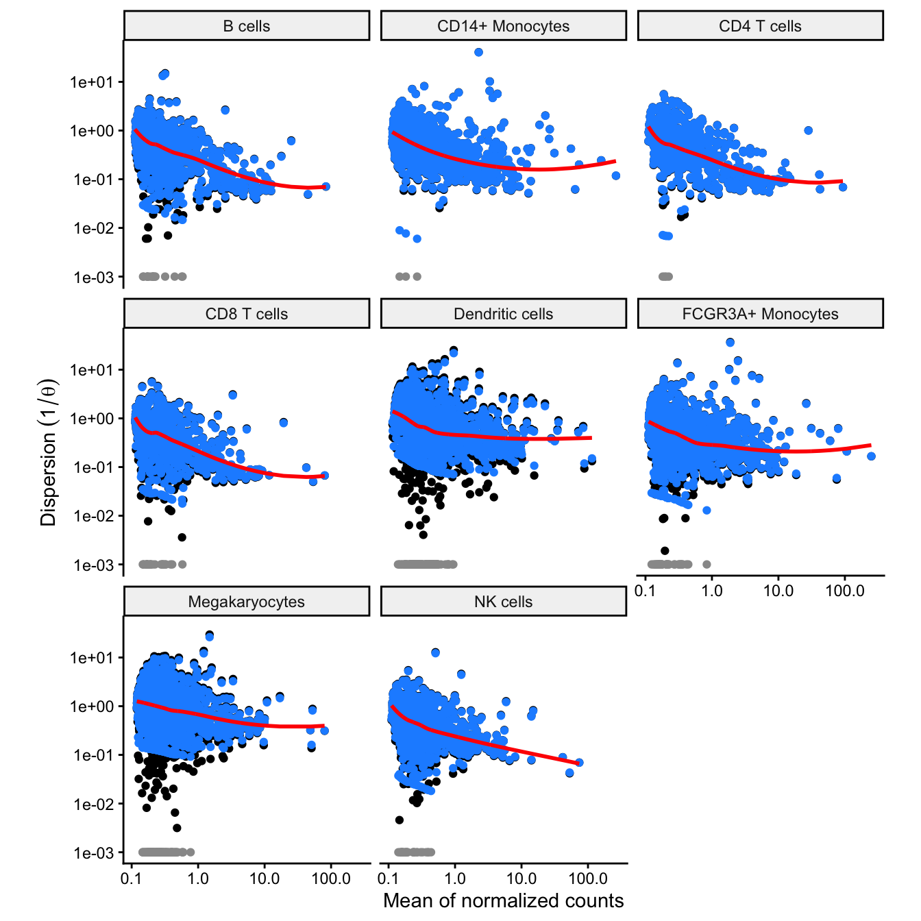
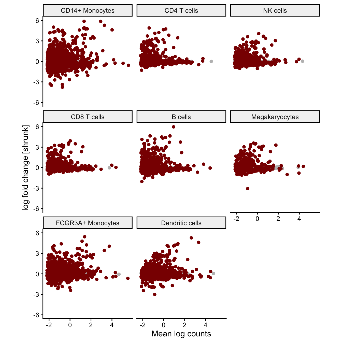
Effect size vs average expression
Plot the relationship between the estimated effect size and mean normalized counts. Genes with low expression have more stochastic variation due to sampling low counts, so their effect size estimates show high variance. The effect sizes should be centered arount zero and the variance should decrease for genes with high counts. Every point is a gene and, genes passing the multiple testing correction are shown in red.
plotMA(fit, coef='Statusstim', ymax=6)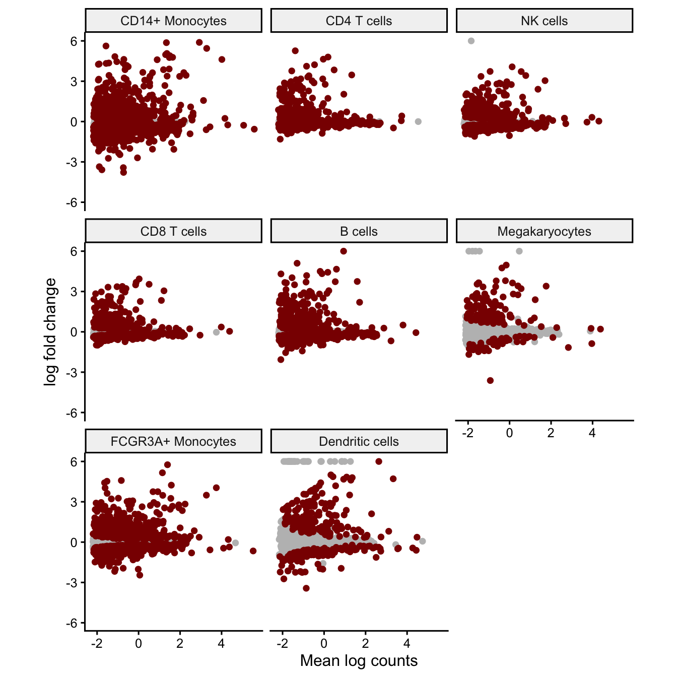
Volcano plot
The volcano plot can indicate the strength of the differential expression signal with each cell type. Genes passing the multiple testing correction are shown in red.
plotVolcano(fit, coef='Statusstim')
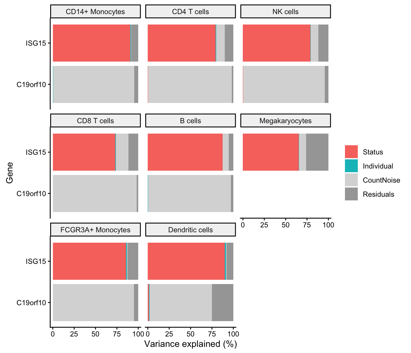
Variance partitioning
Variance partitioning analysis uses linear or linear mixed models to quanify the contribution of multiple sources of expression variation at the gene-level. For each gene it fits a linear (mixed) model and evalutes the fraction of expression variation explained by each variable. Variance fractions can be visualized at the gene-level for each cell type using a bar plot, or genome-wide using a violin plot.
In the case of the NBMM, estimating the variance fractions requires fitting the model again using only an intercept term and the random effect.
Violin plots
fit.null <- lucida(sce, ~ (1|Individual), "CellType")

vp <- fitVarPart(fit, fit.null)

plotVarPart(sortCols(vp))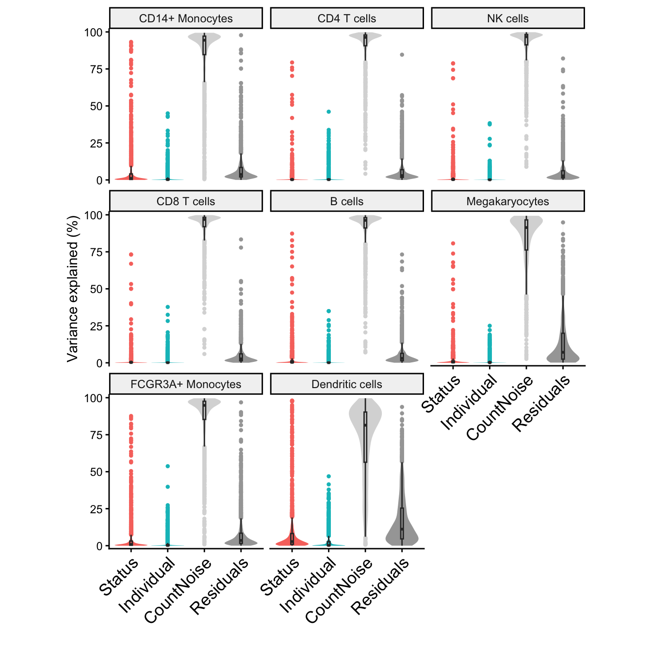
PCA on full dataset
The lucida workflow considers raw counts using a
negative bininomial model. lucida can also transform the
counts for use in downstream analysis like clustering and PCA. Like sctransform (Choudhary and Satija,
2022), lucida can fit a negative binomial model for
each gene across all cell types. A variance stabilizing transform
extract residuals from the model fit to be used for downstream
analysis.
Here, we fit lucida(), extract the deviance residuals,
extract the top 1000 highly variable genes, and then perform out-of-core
SVD with dashSVD(). Principal components reveals the
separation cells based on cell types and stimulation status.
library(GenomicDataStream)

# run lucida using only an intercept
# optionally include technical variables
fit.all <- lucida(sce, ~ 1)

# Evaluate model residuals
res.all <- residuals(fit.all, sce)

# Extract top 1000 highly variable genes
res.hvg <- topHVGs( res.all, fit.all, n = 1000)

# Run out-of-core SVD
pca <- dashSVD(res.hvg, k = 5)

df = pca$v %>%
  data.frame(., CellType = sce$cell, Status = sce$Status)

fig1 = df %>%
  ggplot(aes(PC1, PC2, color=CellType, shape = Status)) +
    geom_point() +
    theme_classic() +
    theme(aspect.ratio=1,
          plot.title = element_text(hjust = 0.5),
          legend.position = "none") +
    xlab("PC 1") +
    ylab("PC 2")

fig2 = df %>%
  ggplot(aes(PC3, PC2, color=CellType, shape = Status)) +
    geom_point() +
    theme_classic() +
    theme(aspect.ratio=1,
          plot.title = element_text(hjust = 0.5)) +
    xlab("PC 3") +
    ylab("PC 2")

fig1 | fig2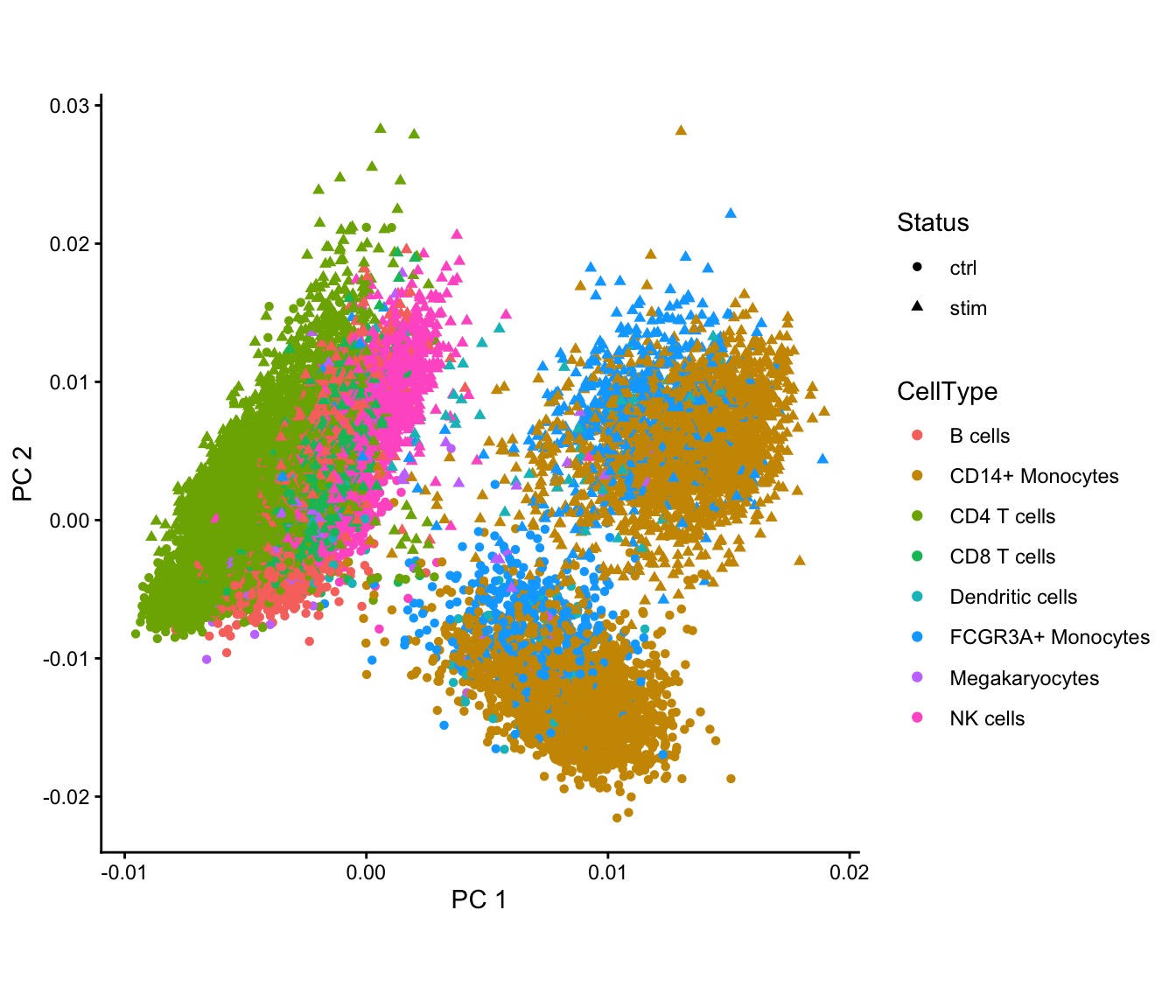
Bayesian post-processing
Setting method = "Bayesian" performs effect size
shrinkage and multiple testing correction using the empirical Bayes
approach of Stephens (2017)
within the ashr package. This reports the local false
discovery rate (lFDR) and the local false sign rate (lFSR). lFDR is the
probability that the true effect size is zero. lFSR is more conservative
and is the estimated probability that the true effect size is has the
opposite sign or is zero.
Extract results
results(fit, coef = "Statusstim", method = "Bayesian")## # A tibble: 9,440 × 9
## cluster_id ID AveExpr logFC se df p.value lFDR lFSR
## <chr> <chr> <dbl> <dbl> <dbl> <dbl> <dbl> <dbl> <dbl>
## 1 CD14+ Monocytes ISG15 55.3 4.62 0.0776 4337. 0 0 0
## 2 CD14+ Monocytes IFI6 3.55 2.68 0.0434 4347. 0 0 0
## 3 CD14+ Monocytes MARCKSL1 2.11 -1.46 0.0365 4347. 8.49e-297 0 0
## 4 CD14+ Monocytes GBP1 1.72 1.93 0.0479 4319. 6.54e-303 0 0
## 5 CD14+ Monocytes RSAD2 4.47 4.76 0.102 4335. 1.00e-286 0 0
## 6 CD14+ Monocytes TMSB10 7.61 1.22 0.0167 4343. 0 0 0
## 7 CD14+ Monocytes RPL15 3.78 -1.01 0.0237 4333. 0 0 0
## 8 CD14+ Monocytes PLSCR1 2.11 1.68 0.0327 4333. 0 0 0
## 9 CD14+ Monocytes TNFSF10 4.51 4.83 0.0884 4321. 6.33e-296 0 0
## 10 CD14+ Monocytes FAM26F 1.71 3.28 0.0781 4331. 4.81e-317 0 0
## # ℹ 9,430 more rowsIn addition, plotMA() and plotVolcano() can
be run with results from Bayesian post-processing.
Volcano plot
plotVolcano(fit, coef='Statusstim', method = "Bayesian")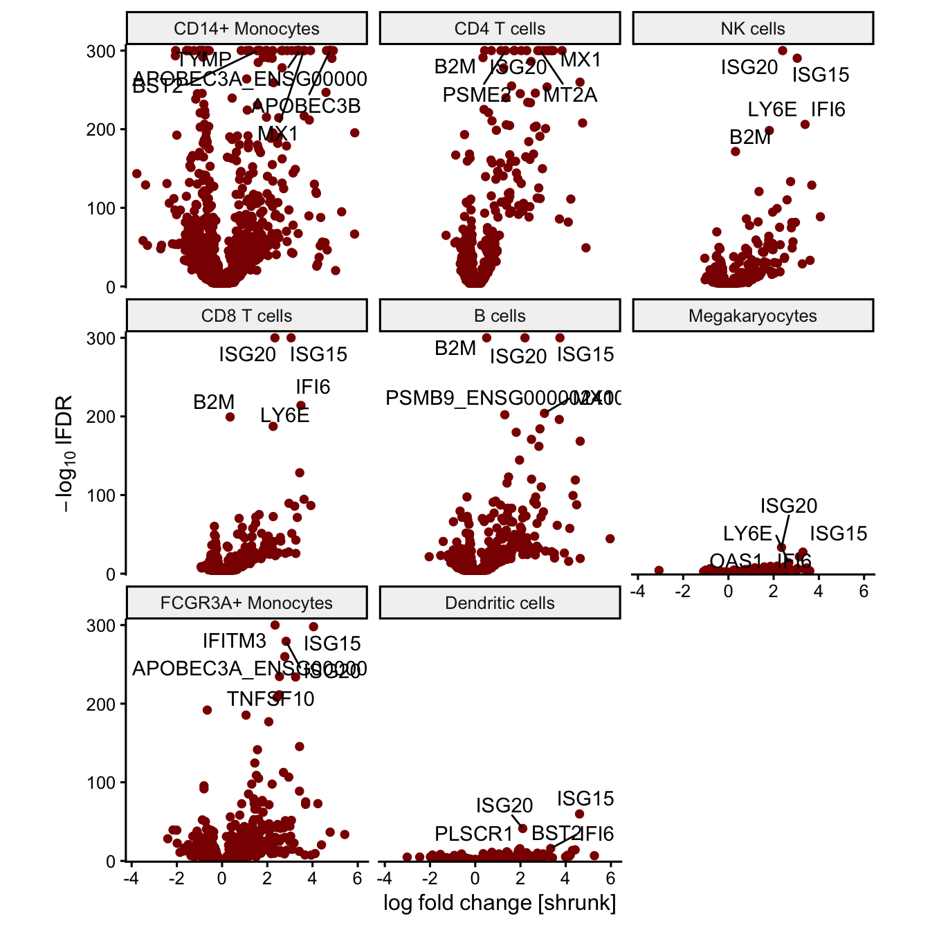
Session info
## R version 4.5.1 (2025-06-13)
## Platform: aarch64-apple-darwin23.6.0
## Running under: macOS Sonoma 14.7.1
##
## Matrix products: default
## BLAS/LAPACK: /opt/homebrew/Cellar/openblas/0.3.33/lib/libopenblasp-r0.3.33.dylib;  LAPACK version 3.12.0
##
## locale:
## [1] en_US.UTF-8/en_US.UTF-8/en_US.UTF-8/C/en_US.UTF-8/en_US.UTF-8
##
## time zone: America/New_York
## tzcode source: internal
##
## attached base packages:
## [1] stats4    stats     graphics  grDevices utils     datasets  methods
## [8] base
##
## other attached packages:
##  [1] GenomicDataStream_0.99.0           muscData_1.24.0
##  [3] aplot_0.2.9                        dplyr_1.2.1
##  [5] scater_1.38.1                      ggplot2_4.0.3
##  [7] scuttle_1.20.0                     ExperimentHub_3.0.0
##  [9] AnnotationHub_4.0.0                BiocFileCache_3.0.0
## [11] dbplyr_2.5.2                       SingleCellExperiment_1.32.0
## [13] SummarizedExperiment_1.40.0        Biobase_2.70.0
## [15] GenomicRanges_1.62.1               Seqinfo_1.0.0
## [17] IRanges_2.44.0                     S4Vectors_0.48.1
## [19] BiocGenerics_0.56.0                generics_0.1.4
## [21] MatrixGenerics_1.22.0              matrixStats_1.5.0
## [23] lucida_0.1.7                       GenomicDataStreamRegression_0.99.2
##
## loaded via a namespace (and not attached):
##   [1] RColorBrewer_1.1-3     jsonlite_2.0.0         magrittr_2.0.5
##   [4] ggbeeswarm_0.7.3       farver_2.1.2           nloptr_2.2.1
##   [7] rmarkdown_2.31         fs_2.1.0               ragg_1.5.2
##  [10] vctrs_0.7.3            memoise_2.0.1          minqa_1.2.8
##  [13] SQUAREM_2026.1         mixsqp_0.3-54          htmltools_0.5.9
##  [16] S4Arrays_1.10.1        progress_1.2.3         curl_7.1.0
##  [19] BiocNeighbors_2.4.0    truncnorm_1.0-9        Rhdf5lib_1.32.0
##  [22] gridGraphics_0.5-1     SparseArray_1.10.10    Formula_1.2-5
##  [25] rhdf5_2.54.1           sass_0.4.10            parallelly_1.47.0
##  [28] bslib_0.11.0           htmlwidgets_1.6.4      desc_1.4.3
##  [31] httr2_1.2.2            cachem_1.1.0           lifecycle_1.0.5
##  [34] pkgconfig_2.0.3        rsvd_1.0.5             Matrix_1.7-5
##  [37] R6_2.6.1               fastmap_1.2.0          anndataR_1.1.3
##  [40] rbibutils_2.4.1        digest_0.6.39          patchwork_1.3.2
##  [43] AnnotationDbi_1.72.0   irlba_2.3.7            textshaping_1.0.5
##  [46] RSQLite_3.52.0         beachmat_2.26.0        labeling_0.4.3
##  [49] invgamma_1.2           filelock_1.0.3         httr_1.4.8
##  [52] abind_1.4-8            compiler_4.5.1         bit64_4.8.0
##  [55] withr_3.0.2            S7_0.2.2               BiocParallel_1.44.0
##  [58] viridis_0.6.5          carData_3.0-6          DBI_1.3.0
##  [61] HDF5Array_1.38.0       MASS_7.3-65            rappdirs_0.3.4
##  [64] DelayedArray_0.36.1    tools_4.5.1            vipor_0.4.7
##  [67] otel_0.2.0             beeswarm_0.4.0         glmGamPoi_1.22.0
##  [70] glue_1.8.1             h5mread_1.2.1          nlme_3.1-169
##  [73] rhdf5filters_1.22.0    grid_4.5.1             gtable_0.3.6
##  [76] tidyr_1.3.2            hms_1.1.4              utf8_1.2.6
##  [79] ScaledMatrix_1.18.0    BiocSingular_1.26.1    car_3.1-5
##  [82] XVector_0.50.0         ggrepel_0.9.8          BiocVersion_3.22.0
##  [85] pillar_1.11.1          stringr_1.6.0          yulab.utils_0.2.4
##  [88] limma_3.66.0           splines_4.5.1          lattice_0.22-9
##  [91] bit_4.6.0              tidyselect_1.2.1       Biostrings_2.78.0
##  [94] knitr_1.51             gridExtra_2.3          reformulas_0.4.4
##  [97] xfun_0.57              statmod_1.5.2          stringi_1.8.7
## [100] ggfun_0.2.0            yaml_2.3.12            boot_1.3-32
## [103] codetools_0.2-20       evaluate_1.0.5         tibble_3.3.1
## [106] BiocManager_1.30.27    ggplotify_0.1.3        cli_3.6.6
## [109] RcppParallel_5.1.11-2  reticulate_1.46.0      pbmcapply_1.5.1
## [112] systemfonts_1.3.2      Rdpack_2.6.6           jquerylib_0.1.4
## [115] BatchRegression_0.0.26 dichromat_2.0-0.1      Rcpp_1.1.1-1.1
## [118] png_0.1-9              parallel_4.5.1         pkgdown_2.2.0
## [121] blob_1.3.0             fastglmm_0.4.7         prettyunits_1.2.0
## [124] beachmat.hdf5_1.8.0    lme4_2.0-1             viridisLite_0.4.3
## [127] scales_1.4.0           purrr_1.2.2            crayon_1.5.3
## [130] fANCOVA_0.6-1          rlang_1.2.0            ashr_2.2-63
## [133] KEGGREST_1.50.0