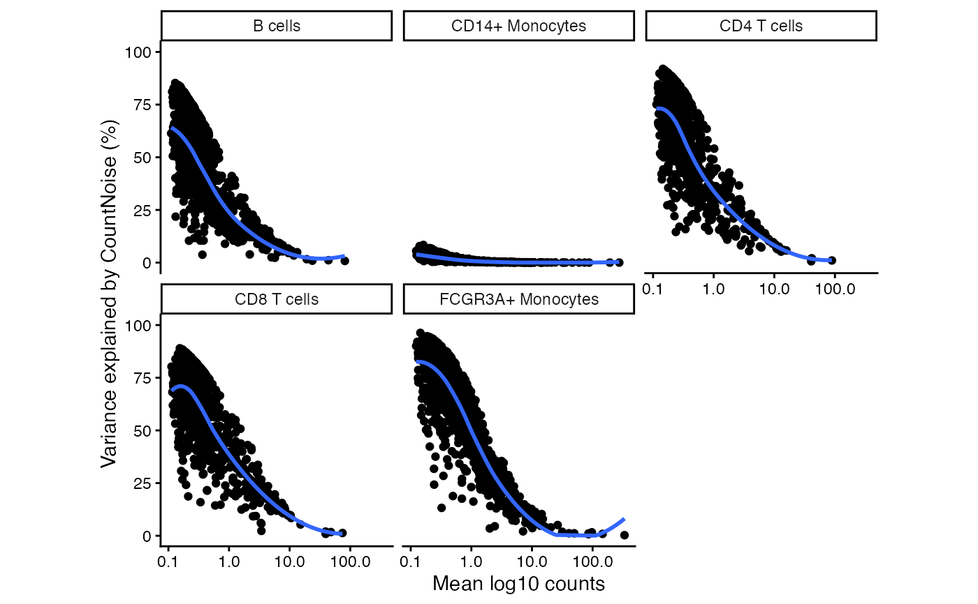
Plot trend of variance fractions for a specified component versus count magnitude for each gene and cell cluster
Arguments
- x
object returned by
lucida()- vp
data.framefromfitVarPart()- component
variance component to extract from
vp- cluster_ids
which cell types to plot
- ...
additional arguments
Examples
library(SingleCellExperiment)

# Load example data
data(example_sce, package="muscat")
sce <- example_sce

# Compute library size for each cell
sce$libSize <- colSums(counts(sce))

# Specify regression formula and cell annotation
form <- ~ group_id + (1|sample_id)
fit <- lucida(sce, form, "cluster_id", verbose=FALSE)
#> B cells
#> CD14+ Monocytes
#> CD4 T cells
#> CD8 T cells
#> FCGR3A+ Monocytes

# Model with only intercept and random effect
form <- ~ (1|sample_id)
fit.null <- lucida(sce, form, "cluster_id", verbose=FALSE)
#> B cells
#> CD14+ Monocytes
#> CD4 T cells
#> CD8 T cells
#> FCGR3A+ Monocytes

# Variance partitioning analysis
vp <- fitVarPart(fit, fit.null)

plotTrendVP(fit, vp, "CountNoise")
#> Warning: Failed to fit group -1.
#> Caused by error in `nls()`:
#> ! step factor 0.000488281 reduced below 'minFactor' of 0.000976562
#> Warning: Failed to fit group -1.
#> Caused by error in `nls()`:
#> ! step factor 0.000488281 reduced below 'minFactor' of 0.000976562
#> Warning: Failed to fit group -1.
#> Caused by error in `nls()`:
#> ! step factor 0.000488281 reduced below 'minFactor' of 0.000976562
#> Warning: Failed to fit group -1.
#> Caused by error in `nls()`:
#> ! step factor 0.000488281 reduced below 'minFactor' of 0.000976562