Plot contrast matrix to clarify interpretation of hypothesis tests with linear contrasts
Details
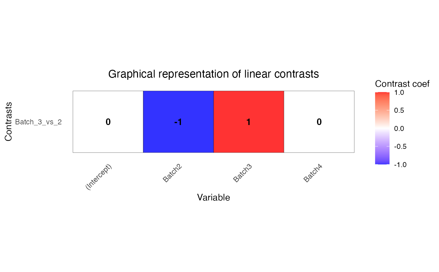
This plot shows the contrasts weights that are applied to each coefficient.
Consider a variable v with levels c('A', 'B', 'C'). A contrast comparing A and B is 'vA - vB' and tests whether the difference between these levels is different than zero. Coded for the 3 levels this has weights c(1, -1, 0). In order to compare A to the other levels, the contrast is 'vA - (vB + vC)/2' so that A is compared to the average of the other two levels. This is encoded as c(1, -0.5, -0.5). This type of proper matching in testing multiple levels is enforced by ensuring that the contrast weights sum to 1. Based on standard regression theory only weighted sums of the estimated coefficients are supported.
Examples
# load library
# library(variancePartition)

# load simulated data:
# geneExpr: matrix of gene expression values
# info: information/metadata about each sample
data(varPartData)

# 1) get contrast matrix testing if the coefficient for Batch2 is different from Batch3
form <- ~ Batch + (1 | Individual) + (1 | Tissue)
L <- makeContrastsDream(form, info, contrasts = c(Batch_3_vs_2 = "Batch3 - Batch2"))

# plot contrasts
plotContrasts(L)