Numerically stable Sidak correction

Compare with other implementations

Developed by Gabriel Hoffman

Run on 2025-07-16 15:51:08

Function to compute using multiple methods

library(ggplot2)
library(tidyverse)
library(sidakCorrection)

sidak <- function(p, n, method = c("adaptive", "double", "mpfr", "taylor"), precBits = 1000) {

    method <- match.arg(method)

    switch(method, double = 1 - (1 - p)^n, mpfr = {
        p_mpfr <- Rmpfr::mpfr(p, precBits = precBits)
        as.numeric(1 - (1 - p_mpfr)^as.integer(n))
    }, taylor = {
        # Set the cutoff to be 1, so the Taylor series is always used
        sidakCorrection(p, n, 1)
    }, adaptive = {
        sidakCorrection(p, n)
    })
}

Example for single p-values

p = 1e-18
n = 1e+05

sidak(p, n, "double")

## [1] 0

sidak(p, n, "mpfr")

## [1] 1e-13

sidak(p, n, "taylor")

## [1] 1e-13

sidak(p, n, "adaptive")

## [1] 1e-13

Compare methods

Here we plot the values from computing the Sidak correction using

• adaptive approach using either double precision or Taylor series depending on the value of p
• High precision with Rmpfr
• standard approach using double precision arithmetic
• Taylor series

x = 10^-seq(0, 20, length.out = 100)

df = tibble(x = x, `Standard (double)` = sidak(x, n, "double"), `High precision (mpfr)` = sidak(x,
    n, "mpfr", 1000), `Taylor series` = sidak(x, n, "taylor"), Adaptive = sidak(x,
    n, "adaptive")) %>%
    pivot_longer(!x)

df %>%
    ggplot(aes(x, value, color = name, linetype = name)) + geom_line(linewidth = 2) +
    theme_classic() + theme(aspect.ratio = 1) + scale_x_log10() + scale_y_log10(limits = c(1e-19,
    1000)) + xlab("Input p-value (log10 scale)") + ylab("Sidak corrected p-value (log10 scale)")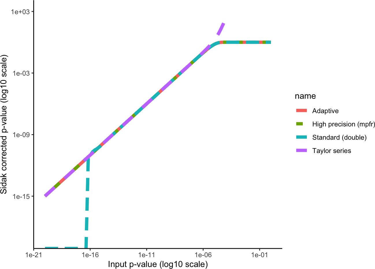

We see that the double precision approach deviates from the high precision method for small values of p, while the Taylor series deviates for large values of p. The adpative approach used bo the sidakCorrection() function matches that high precision method.