Test differential variance

Test the association between a covariate of interest and the response's deviation from expectation.

Usage

# S4 method for dreamletResult
diffVar(
  fit,
  method = c("AD", "SQ"),
  scale = c("leverage", "none"),
  BPPARAM = SerialParam(),
  ...
)

Arguments

fit: model fit from dream()
method: transform the residuals using absolute deviation ("AD") or squared deviation ("SQ").
scale: scale each observation by "leverage", or no scaling ("none")
BPPARAM: parameters for parallel evaluation
...: other parameters passed to dream()

Details

This method performs a test of differential variance between two subsets of the data, in a way that generalizes to multiple categories, continuous variables and metrics of spread beyond variance. For the two category test, this method is simular to Levene's test. This model was adapted from Phipson, et al (2014), extended to linear mixed models, and adapted to be compatible with variancePartition::dream() and dreamlet::dreamlet().

This method is composed of multiple steps where 1) a typical linear (mixed) model is fit with dreamlet(), 2) residuals are computed and transformed based on an absolute value or squaring transform, 3) a second regression is performed with dreamlet() to test if a variable is associated with increased deviation from expectation. Both regression take advantage of the dreamlet() linear (mixed) modelling framework followed by empirical Bayes shrinkage that extends the limma::voom() framework.

Note that diffVar() takes the results of the first regression as a parameter to use as a starting point.

References

Phipson B, Oshlack A (2014). “DiffVar: a new method for detecting differential variability with application to methylation in cancer and aging.” Genome biology, 15(9), 1--16.

Examples

library(muscat)
library(SingleCellExperiment)

data(example_sce)

# create pseudobulk for each sample and cell cluster
pb <- aggregateToPseudoBulk(example_sce,
  assay = "counts",
  cluster_id = "cluster_id",
  sample_id = "sample_id",
  verbose = FALSE
)

# voom-style normalization
res.proc <- processAssays(pb, ~group_id)
#>   B cells...
#> 0.13 secs
#>   CD14+ Monocytes...
#> 0.21 secs
#>   CD4 T cells...
#> 0.15 secs
#>   CD8 T cells...
#> 0.078 secs
#>   FCGR3A+ Monocytes...
#> 0.18 secs

# Differential expression analysis within each assay,
# evaluated on the voom normalized data
res.dl <- dreamlet(res.proc, ~group_id)
#>   B cells...
#> 0.093 secs
#>   CD14+ Monocytes...
#> 0.12 secs
#>   CD4 T cells...
#> 0.1 secs
#>   CD8 T cells...
#> 0.059 secs
#>   FCGR3A+ Monocytes...
#> 0.13 secs

# Differential variance analysis
# result is a dreamlet fit
res.dvar <- diffVar(res.dl)

# Examine results
res.dvar
#> class: dreamletResult 
#> assays(5): B cells CD14+ Monocytes CD4 T cells CD8 T cells FCGR3A+
#>   Monocytes
#> Genes:
#>  min: 531 
#>  max: 1130 
#> details(7): assay n_retain ... n_errors error_initial
#> coefNames(2): (Intercept) group_idstim

# Examine details for each assay
details(res.dvar)
#>               assay n_retain   formula formDropsTerms n_genes n_errors
#> 1           B cells        4 ~group_id          FALSE     847        0
#> 2   CD14+ Monocytes        4 ~group_id          FALSE    1130        0
#> 3       CD4 T cells        4 ~group_id          FALSE     897        0
#> 4       CD8 T cells        4 ~group_id          FALSE     531        0
#> 5 FCGR3A+ Monocytes        4 ~group_id          FALSE    1086        0
#>   error_initial
#> 1         FALSE
#> 2         FALSE
#> 3         FALSE
#> 4         FALSE
#> 5         FALSE

# show coefficients estimated for each cell type
coefNames(res.dvar)
#> [1] "(Intercept)"  "group_idstim"

# extract results using limma-style syntax
# combines all cell types together
# adj.P.Val gives study-wide FDR
topTable(res.dvar, coef = "group_idstim", number = 3)
#> DataFrame with 3 rows and 9 columns
#>         assay          ID     logFC   AveExpr         t     P.Value   adj.P.Val
#>   <character> <character> <numeric> <numeric> <numeric>   <numeric>   <numeric>
#> 1 CD4 T cells     DYNLRB1  0.978587  0.525150   1179.42 1.28303e-11 1.91186e-08
#> 2 CD4 T cells       RNPS1  1.103936  0.686623   1002.75 2.36305e-11 1.91186e-08
#> 3 CD4 T cells       SLFN5  0.818186  0.444949    964.08 2.74004e-11 1.91186e-08
#>           B     z.std
#>   <numeric> <numeric>
#> 1   18.1794   1179.42
#> 2   17.6567   1002.75
#> 3   17.5220    964.08

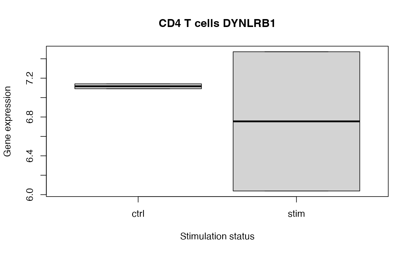
# Plot top hit to see differential variance
# Note that this is a toy example with only 4 samples
cellType <- "CD4 T cells"
gene <- "DYNLRB1"

y <- res.proc[[cellType]]$E[gene, ]
x <- colData(res.proc)$group_id

boxplot(y ~ x,
  xlab = "Stimulation status",
  ylab = "Gene expression",
  main = paste(cellType, gene)
)

#

Usage

Arguments

Details

References

See also

Examples