Window-based Randomized SVD

Usage

PCAstream(
  x,
  k,
  ...,
  p = 7,
  s = 20,
  B = 64,
  threads = 4,
  threads2 = 4,
  scaleAndCenter = TRUE,
  shuffle = TRUE,
  verbose = TRUE
)

# S4 method for class 'GenomicDataStream'
PCAstream(
  x,
  k,
  ...,
  p = 7,
  s = 20,
  B = 64,
  threads = 4,
  threads2 = 1,
  scaleAndCenter = TRUE,
  shuffle = TRUE,
  verbose = TRUE
)

# S4 method for class 'ANY'
PCAstream(
  x,
  k,
  chunkSize = 1000,
  p = 7,
  s = 20,
  B = 64,
  threads = 4,
  threads2 = 4,
  scaleAndCenter = TRUE,
  shuffle = TRUE,
  verbose = TRUE
)

# S4 method for class 'SummarizedExperiment'
PCAstream(
  x,
  k,
  chunkSize = 1000,
  assay = "logcounts",
  ...,
  p = 7,
  s = 20,
  B = 64,
  threads = 4,
  threads2 = 4,
  scaleAndCenter = TRUE,
  shuffle = TRUE,
  verbose = TRUE
)

Arguments

x: GenomicDataStream, or matrix as matrix, DelayedArray.
k: integer;
specifies the target rank of the low-rank decomposition. \(k\) should satisfy \(k << min(m,n)\).
...: other argument to control streaming
p: integer, optional;
number of additional power iterations (by default \(p=7\)).
s: integer, optional;
oversampling parameter (by default \(s=20\)).
B: integer, optional;
number of windows (by default \(B=64\)).
threads: integer, optional;
number of threads (by default \(threads=4\)) to read data
threads2: integer, optional;
number of threads (by default \(threads=4\)), used for linear algebra opertions
scaleAndCenter: bool, optional;
if TRUE, scale and center features
shuffle: bool, optional;
if TRUE (default) shuffle genomic regions, the next chunk is not in LD with the previous chunk
verbose: string, optional;
if TRUE (default), print details
chunkSize: number of features to read per chunk in GenomicDataStream
assay: for SummarizedExperiment which assay to perform PCA on

Value

PCAstream returns a list containing the following three components:

d: array_like;
singular values; vector of length \((k)\).
u: array_like;
left singular vectors; \((m, k)\) or \((m, nu)\) dimensional array.
v: array_like;
right singular vectors; \((n, k)\) or \((n, nv)\) dimensional array.

Details

PCAstream implements the window-based Randomized SVD proposed by Li, et al. (2023).

If scaleAndCenter, the data matrix is scaled so that each feature has a mean of zero and a cross-product of 1. In this case the sum of squares of all eigen values equals the number of features (i.e sum(d^2) = p).

Computational time is spent on two steps:

1) Reading data from disk and and processing data. Multiple chunks can be read and processed in parallel. This is conrolled by setting threads

2) Updating PCA with current data chunk. Only one chunk can be processed at a time, but linear algebra operations can be parallelized. This is conrolled by setting threads2

If x is a matrix, PCA is performed using rows as features. Note: this is the _transpose_ of what svd() does.

Note

The singular vectors are not unique and only defined up to sign. If a left singular vector has its sign changed, changing the sign of the corresponding right vector gives an equivalent decomposition.

References

Li, Z., Meisner, J., & Albrechtsen, A. (2023). Fast and accurate out-of-core PCA framework for large scale biobank data. Genome Research, 33(9), 1599-1608. doi:10.1101/gr.277525.122 .

Author

Zilong Li zilong.dk@gmail.com, Gabriel Hoffman

Examples

# Example: PCA on genotype data
file <- system.file("extdata", "test.vcf.gz", package = "GenomicDataStream")

obj <- GenomicDataStream(file, "DS", chunkSize = 3)

res <- PCAstream(obj, k=5, threads=1)
#> Read through...
#>  # features: 10
#>  # chunks: 2
#>  # PCs: 5
#>  # threads: 1
#> 
Epoch 0 / 7  
Epoch 1 / 7  
Epoch 2 / 7  
Epoch 3 / 7  
Epoch 4 / 7  
Epoch 5 / 7  
Epoch 6 / 7  
Epoch 7 / 7  
Final decompositions
Completed            

res
#> 
#>        PCA: Computed first 5 PCs
#> 
#>  $u
#>           PC1         PC2         PC3
#> I1 -0.2195584 -0.02863333 -0.14971387
#> I2 -0.1518848 -0.03797283  0.05389429
#>      ...
#> 
#>  $v
#>                     PC1        PC2          PC3
#> 1:10000:C:A -0.53910201 -0.1405398 -0.007546938
#> 1:11000:T:C -0.07783198  0.1641358 -0.288227120
#>      ...
#> 
#>  $d
#> 1.276828 1.189663 ...
#> 

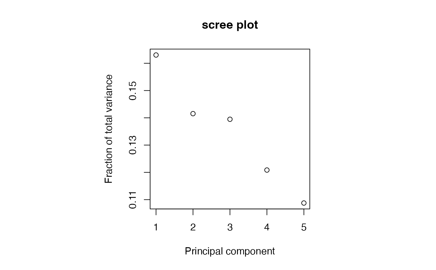
par(pty="s")
plot(res)


# Example: PCA on gene expression data
library(muscat)
library(SingleCellExperiment)
library(GenomicDataStream) 

data(example_sce)
sce <- example_sce

# Normalize expression with log2 counts per million
prior.count <- 1
lib.size <- colSums2(counts(sce))
logcounts(sce) <- t(log2(t(counts(sce) + prior.count)) - log2(lib.size) + log2(1e6))

# PCA on SingleCellExperiment with assay logcounts
res <- PCAstream(sce, k=5, assay="logcounts")
#> Scale and centering...
#> 
Epoch 0 / 7  
Epoch 1 / 7  
Epoch 2 / 7  
Epoch 3 / 7  
Epoch 4 / 7  
Epoch 5 / 7  
Epoch 6 / 7  
Epoch 7 / 7  
Final decompositions
Completed            

res
#> 
#>        PCA: Computed first 5 PCs
#> 
#>  $u
#>                          PC1          PC2           PC3
#> ATCATGCTGCGTAT-1 -0.02663795 -0.004300371 -0.0108049057
#> GTACGAACTGTCAG-1 -0.01792728  0.011907831 -0.0007039027
#>      ...
#> 
#>  $v
#>                PC1         PC2        PC3
#> HES4  -0.029479111 -0.03760661 0.02539624
#> ISG15  0.004348096 -0.09931692 0.09957708
#>      ...
#> 
#>  $d
#> 26.88395 7.028332 ...
#>